Extract features from CSLs

After creating and annotating CSLs, features can be extracted from each cell to quantitatively compare molecular intensity differences and spatial re-localisation of proteins in different conditions. CAMPA can extract the following features:

• Intensity: per-cluster mean and size features. Needs to be calculated first to set up the adata.

• Co-occurrence: spatial co-occurrence between pairs of clusters at different distances.

• Object stats: number and area of connected components per cluster

The features are saved as an AnnData object and can be used to compare molecular abundance within CSLs and spatial co-occurrence of CSLs in different conditions (e.g. perturbations).

Please make sure that you clustered the data and projected the result to the entire example dataset as described in the Cluster data into CSLs tutorial before running this tutorial.

from pathlib import Path
import os

from IPython.display import display
import pandas as pd
import anndata as ad

from campa.pl import (
    plot_mean_size,
    plot_object_stats,
    plot_co_occurrence,
    plot_mean_intensity,
    get_intensity_change,
    plot_intensity_change,
    plot_co_occurrence_grid,
)
from campa.tl import Experiment, extract_features, FeatureExtractor
from campa.utils import load_config, init_logging, merged_config
from campa.constants import campa_config

# init logging with level INFO=20, WARNING=30
init_logging(level=30)
# read correct campa_config -- created with setup.ipynb
CAMPA_DIR = Path.cwd()
campa_config.config_fname = CAMPA_DIR / "params/campa.ini"
print(campa_config)

2022-11-25 14:34:34.778284: I tensorflow/core/platform/cpu_feature_guard.cc:193] This TensorFlow binary is optimized with oneAPI Deep Neural Network Library (oneDNN) to use the following CPU instructions in performance-critical operations:  AVX2 AVX512F AVX512_VNNI FMA
To enable them in other operations, rebuild TensorFlow with the appropriate compiler flags.
2022-11-25 14:34:52.031324: I tensorflow/core/util/util.cc:169] oneDNN custom operations are on. You may see slightly different numerical results due to floating-point round-off errors from different computation orders. To turn them off, set the environment variable `TF_ENABLE_ONEDNN_OPTS=0`.
2022-11-25 14:34:55.054866: E tensorflow/stream_executor/cuda/cuda_blas.cc:2981] Unable to register cuBLAS factory: Attempting to register factory for plugin cuBLAS when one has already been registered

Reading config from /home/icb/hannah.spitzer/projects/pelkmans/software_new/campa_notebooks_test/params/campa.ini
CAMPAConfig (fname: /home/icb/hannah.spitzer/projects/pelkmans/software_new/campa_notebooks_test/params/campa.ini)
EXPERIMENT_DIR: /home/icb/hannah.spitzer/projects/pelkmans/software_new/campa_notebooks_test/example_experiments
BASE_DATA_DIR: /home/icb/hannah.spitzer/projects/pelkmans/software_new/campa_notebooks_test/example_data
CO_OCC_CHUNK_SIZE: 10000000.0
data_config/exampledata: /home/icb/hannah.spitzer/projects/pelkmans/software_new/campa_notebooks_test/params/ExampleData_constants.py

Extract features

To extract features, the high-level API function extract_features is used.

Extracting co-occurrence scores can take a long time, and it is recommended to use the CLI to run the feature extraction in a script:

cd CAMPA_DIR/params
campa extract_features example_feature_params.py

To define which features should be extracted, a parameter dictionary is used. All parameters that can be set in this dictionary are documented with the extract_features function. Here, we are going to use an example feature params file that extracts intensity, co-occurrence, and object features (object size, circularity, etc.) from the test_pre_trained/CondVAE_pert-CC experiment we clustered in the clustering tutorial.

# load parameter dictionary
params = load_config("params/example_feature_params.py")
# just use the first variable_params configuration here
for variable_params in params.variable_feature_params[:1]:
    cur_params = merged_config(params.feature_params, variable_params)
print(cur_params)

{'experiment_dir': 'test_pre_trained/CondVAE_pert-CC', 'cluster_name': 'clustering_res0.2', 'cluster_dir': 'aggregated/sub-pre', 'cluster_col': 'annotation', 'data_dirs': ['184A1_unperturbed/I09', '184A1_unperturbed/I11', '184A1_meayamycin/I12', '184A1_meayamycin/I20'], 'save_name': 'features_annotation.h5ad', 'force': False, 'features': ['intensity', 'co-occurrence', 'object-stats'], 'co_occurrence_params': {'min': 2.0, 'max': 60.0, 'nsteps': 5, 'logspace': True, 'num_processes': None}, 'object_stats_params': {'features': ['area', 'circularity', 'elongation', 'extent'], 'channels': []}}

Using these parameters, we can now extract the features. The extracted features will be saved to cur_params['save_name'] in each data directory in experiment_dir/aggregated/full_data.

Note that this step will take ~10 minutes to complete. For a faster result, you can turn off the computation of the co-occurrence features by setting cur_params['features'] = ['intensity', 'object-stats']

extract_features(cur_params)

Cannot read with memmap:  /home/icb/hannah.spitzer/projects/pelkmans/software_new/campa_notebooks_test/example_experiments/test_pre_trained/CondVAE_pert-CC/aggregated/full_data/184A1_unperturbed/I09/clustering_res0.2.npy
Cannot read with memmap:  /home/icb/hannah.spitzer/projects/pelkmans/software_new/campa_notebooks_test/example_experiments/test_pre_trained/CondVAE_pert-CC/aggregated/full_data/184A1_unperturbed/I11/clustering_res0.2.npy
Cannot read with memmap:  /home/icb/hannah.spitzer/projects/pelkmans/software_new/campa_notebooks_test/example_experiments/test_pre_trained/CondVAE_pert-CC/aggregated/full_data/184A1_meayamycin/I12/clustering_res0.2.npy
Cannot read with memmap:  /home/icb/hannah.spitzer/projects/pelkmans/software_new/campa_notebooks_test/example_experiments/test_pre_trained/CondVAE_pert-CC/aggregated/full_data/184A1_meayamycin/I20/clustering_res0.2.npy

Explore and plot extracted features

Features are stored in AnnData objects with obs=cells and vars=channels. Intensity information is stored as layers, co-occurrence scores as obsm matrices (obs x distances for each cluster-cluster pair), and object features as matrices in uns.

The FeatureExtractor class loads this AnnData object and provides convenience functions to access feature information.

# load features for each data_dir
exp = Experiment.from_dir("test_pre_trained/CondVAE_pert-CC")
extrs = [
    FeatureExtractor.from_adata(
        os.path.join(exp.full_path, "aggregated/full_data", data_dir, "features_annotation.h5ad")
    )
    for data_dir in exp.data_params["data_dirs"]
]

extrs[0].adata

AnnData object with n_obs × n_vars = 12 × 34
    obs: 'mapobject_id', 'plate_name', 'well_name', 'well_pos_y', 'well_pos_x', 'tpoint', 'zplane', 'label', 'is_border', 'mapobject_id_cell', 'plate_name_cell', 'well_name_cell', 'well_pos_y_cell', 'well_pos_x_cell', 'tpoint_cell', 'zplane_cell', 'label_cell', 'is_border_cell', 'is_mitotic', 'is_mitotic_labels', 'is_polynuclei_HeLa', 'is_polynuclei_HeLa_labels', 'is_polynuclei_184A1', 'is_polynuclei_184A1_labels', 'is_SBF2_Sphase_labels', 'is_SBF2_Sphase', 'Heatmap-48', 'cell_cycle', 'description', 'dimensions', 'id', 'cell_type', 'EU', 'duration', 'perturbation', 'secondary_only', 'siRNA', 'perturbation_duration', 'LocalDensity_Nuclei_800', 'TR_factor', 'TR_norm', 'TR', 'TR_factor_DMSO-unperturbed', 'TR_norm_DMSO-unperturbed', 'obj_id_int'
    uns: 'clusters', 'co_occurrence_params', 'object_stats', 'object_stats_params', 'params'
    obsm: 'co_occurrence_Nuclear speckles_Nuclear speckles', 'co_occurrence_Nuclear speckles_Nucleolus', 'co_occurrence_Nuclear speckles_Nucleoplasm', 'co_occurrence_Nuclear speckles_PML bodies', 'co_occurrence_Nucleolus_Nuclear speckles', 'co_occurrence_Nucleolus_Nucleolus', 'co_occurrence_Nucleolus_Nucleoplasm', 'co_occurrence_Nucleolus_PML bodies', 'co_occurrence_Nucleoplasm_Nuclear speckles', 'co_occurrence_Nucleoplasm_Nucleolus', 'co_occurrence_Nucleoplasm_Nucleoplasm', 'co_occurrence_Nucleoplasm_PML bodies', 'co_occurrence_PML bodies_Nuclear speckles', 'co_occurrence_PML bodies_Nucleolus', 'co_occurrence_PML bodies_Nucleoplasm', 'co_occurrence_PML bodies_PML bodies', 'size'
    layers: 'intensity_Nuclear speckles', 'intensity_Nucleolus', 'intensity_Nucleoplasm', 'intensity_PML bodies'

The AnnData object contains all feature information

extr = extrs[0]
print("AnnData read from", extr.fname)
print(extr.adata)

AnnData read from /home/icb/hannah.spitzer/projects/pelkmans/software_new/campa_notebooks_test/example_experiments/test_pre_trained/CondVAE_pert-CC/aggregated/full_data/184A1_unperturbed/I09/features_annotation.h5ad
AnnData object with n_obs × n_vars = 12 × 34
    obs: 'mapobject_id', 'plate_name', 'well_name', 'well_pos_y', 'well_pos_x', 'tpoint', 'zplane', 'label', 'is_border', 'mapobject_id_cell', 'plate_name_cell', 'well_name_cell', 'well_pos_y_cell', 'well_pos_x_cell', 'tpoint_cell', 'zplane_cell', 'label_cell', 'is_border_cell', 'is_mitotic', 'is_mitotic_labels', 'is_polynuclei_HeLa', 'is_polynuclei_HeLa_labels', 'is_polynuclei_184A1', 'is_polynuclei_184A1_labels', 'is_SBF2_Sphase_labels', 'is_SBF2_Sphase', 'Heatmap-48', 'cell_cycle', 'description', 'dimensions', 'id', 'cell_type', 'EU', 'duration', 'perturbation', 'secondary_only', 'siRNA', 'perturbation_duration', 'LocalDensity_Nuclei_800', 'TR_factor', 'TR_norm', 'TR', 'TR_factor_DMSO-unperturbed', 'TR_norm_DMSO-unperturbed', 'obj_id_int'
    uns: 'clusters', 'co_occurrence_params', 'object_stats', 'object_stats_params', 'params'
    obsm: 'co_occurrence_Nuclear speckles_Nuclear speckles', 'co_occurrence_Nuclear speckles_Nucleolus', 'co_occurrence_Nuclear speckles_Nucleoplasm', 'co_occurrence_Nuclear speckles_PML bodies', 'co_occurrence_Nucleolus_Nuclear speckles', 'co_occurrence_Nucleolus_Nucleolus', 'co_occurrence_Nucleolus_Nucleoplasm', 'co_occurrence_Nucleolus_PML bodies', 'co_occurrence_Nucleoplasm_Nuclear speckles', 'co_occurrence_Nucleoplasm_Nucleolus', 'co_occurrence_Nucleoplasm_Nucleoplasm', 'co_occurrence_Nucleoplasm_PML bodies', 'co_occurrence_PML bodies_Nuclear speckles', 'co_occurrence_PML bodies_Nucleolus', 'co_occurrence_PML bodies_Nucleoplasm', 'co_occurrence_PML bodies_PML bodies', 'size'
    layers: 'intensity_Nuclear speckles', 'intensity_Nucleolus', 'intensity_Nucleoplasm', 'intensity_PML bodies'

Intensity features

Intensity features are the mean intensity of channels in each cluster (CSL).

Intensity information for each CSL is contained in a separate layer in FeatureExtractor.adata.layers. Overall (per cell) intensity information is stored in FeatureExtractor.adata.X. In addition to the mean intensity per CSL, the adata also contains the size of each CSL per cell in FeatureExtractor.adata.obsm['size']

# intensity per CSL
print("Intensity per CLS stored in", extr.adata.layers)

# whole cell intensity
print("Whole cell intensity stored in X with shape", extr.adata.X.shape)

# size of CSLs per cell
display(extr.adata.obsm["size"])

Intensity per CLS stored in Layers with keys: intensity_Nuclear speckles, intensity_Nucleolus, intensity_Nucleoplasm, intensity_PML bodies
Whole cell intensity stored in X with shape (12, 34)

	all	Nuclear speckles	Nucleolus	Nucleoplasm	PML bodies
0	13668	1237.0	3090	9058	283
1	14816	1385.0	3457	9477	497
2	13048	1318.0	2384	8424	922
3	13478	890.0	2629	9475	484
4	22785	1202.0	5749	15396	438
5	6876	35.0	50	6580	211
6	10961	1081.0	1918	7760	202
7	10340	738.0	2120	7243	239
8	9010	0.0	367	8460	183
9	14668	841.0	2898	10590	339
10	10472	616.0	2091	7414	351
11	13547	1363.0	2807	9003	374

It is possible to export the intensity information in one csv file using FeatureExtractor.extract_intensity_csv. The resulting csv file contains the intensity per CSL for each channel as columns, with CSLs stacked on top of each other, as well as additionally defined columns. This saves a csv file in experiment_dir/aggregated/full_data/data_dir/export.

for extr in extrs:
    extr.extract_intensity_csv(obs=["well_name", "perturbation_duration", "TR"])

extr = extrs[0]
# check if results are stored
save_dir = os.path.join(os.path.dirname(extr.fname), "export")
print("csv exported to", save_dir)
print([n for n in os.listdir(save_dir) if "intensity" in n])

display(pd.read_csv(os.path.join(save_dir, "intensity_features_annotation.csv"), index_col=0))

csv exported to /home/icb/hannah.spitzer/projects/pelkmans/software_new/campa_notebooks_test/example_experiments/test_pre_trained/CondVAE_pert-CC/aggregated/full_data/184A1_unperturbed/I09/export
['intensity_features_annotation.csv']

	01_CDK9_pT186	01_PABPC1	02_CDK7	03_CDK9	03_RPS6	05_GTF2B	05_Sm	07_POLR2A	07_SETD1A	08_H3K4me3	...	21_COIL	21_NCL	00_DAPI	07_H2B	size	cluster	mapobject_id	well_name	perturbation_duration	TR
0	0.220263	0.168692	0.292341	0.227046	0.344410	0.400212	0.351876	0.268362	0.197742	0.309594	...	0.347049	0.205577	0.420119	0.692879	13668.0	all	205776	I09	normal	357.672008
1	0.333146	0.382737	0.403504	0.367799	0.526189	0.556079	0.402247	0.302671	0.285122	0.310469	...	0.350691	0.278747	0.379324	0.583052	14816.0	all	205790	I09	normal	428.364268
2	0.360394	0.480734	0.525491	0.355149	0.551694	0.361255	0.403097	0.348874	0.319844	0.488086	...	0.413549	0.186384	0.419490	0.477315	13048.0	all	248082	I09	normal	250.488581
3	0.374549	0.272541	0.386451	0.359641	0.469129	0.475133	0.340987	0.407483	0.261632	0.405096	...	0.317883	0.197697	0.611018	0.500728	13478.0	all	248102	I09	normal	515.735421
4	0.274677	0.239059	0.358933	0.218737	0.355724	0.362768	0.262636	0.304999	0.315362	0.348737	...	0.267697	0.157225	0.522850	0.360451	22785.0	all	259784	I09	normal	348.150713
5	0.545745	0.589634	0.538518	0.790598	0.812851	0.687019	0.353689	0.564811	0.273066	0.620842	...	0.586261	0.291767	0.744431	0.661208	6876.0	all	291041	I09	normal	443.565445
6	0.225679	0.147178	0.287102	0.215611	0.330553	0.347149	0.258178	0.152336	0.079622	0.224427	...	0.339826	0.172255	0.536892	0.787214	10961.0	all	345908	I09	normal	316.004105
7	0.297851	0.296048	0.432829	0.343467	0.484858	0.489976	0.353426	0.433215	0.270189	0.437530	...	0.362085	0.221666	0.534294	0.665742	10340.0	all	359378	I09	normal	367.904255
8	0.345589	0.388527	0.627053	0.528497	0.576135	0.671750	0.336406	0.337385	0.116071	0.348818	...	0.568719	0.287813	0.669855	0.795703	9010.0	all	359393	I09	normal	513.668590
9	0.187118	0.153416	0.287734	0.215821	0.270915	0.352462	0.278277	0.222176	0.141322	0.275406	...	0.307268	0.177784	0.418376	0.527903	14668.0	all	366493	I09	normal	330.847832
10	0.462329	0.304857	0.561744	0.448209	0.551895	0.686498	0.407504	0.552158	0.333329	0.504888	...	0.478053	0.263166	0.483056	0.613083	10472.0	all	383341	I09	normal	388.012319
11	0.294427	0.227145	0.373680	0.315884	0.373401	0.480220	0.350587	0.404187	0.261491	0.322150	...	0.338741	0.187825	0.408714	0.661022	13547.0	all	383793	I09	normal	376.243596
12	0.507860	0.116696	0.415587	0.411071	0.269115	0.466287	0.647966	0.425061	0.430787	0.434477	...	0.551629	0.068284	0.344541	0.637030	1237.0	Nuclear speckles	205776	I09	normal	357.672008
13	0.623703	0.458236	0.522437	0.621646	0.584039	0.634695	0.659342	0.454861	0.618518	0.423877	...	0.551859	0.140339	0.320592	0.544304	1385.0	Nuclear speckles	205790	I09	normal	428.364268
14	0.682698	0.406474	0.678200	0.579281	0.511746	0.443788	0.689661	0.466248	0.635434	0.669755	...	0.534957	0.111079	0.382885	0.477689	1318.0	Nuclear speckles	248082	I09	normal	250.488581
15	0.829828	0.228499	0.542535	0.664138	0.394651	0.567538	0.591148	0.610244	0.561811	0.564465	...	0.539236	0.097210	0.560445	0.503501	890.0	Nuclear speckles	248102	I09	normal	515.735421
16	0.587949	0.200030	0.538934	0.374302	0.298699	0.427932	0.459766	0.409769	0.776006	0.492420	...	0.392491	0.074476	0.402964	0.293739	1202.0	Nuclear speckles	259784	I09	normal	348.150713
17	0.879115	0.505580	0.859152	1.269043	0.678345	0.870895	0.349357	0.862588	0.409897	0.872185	...	0.627324	0.347079	0.843770	0.665566	35.0	Nuclear speckles	291041	I09	normal	443.565445
18	0.436311	0.122306	0.363612	0.341447	0.301133	0.391417	0.435425	0.200541	0.132738	0.296614	...	0.507728	0.064535	0.437343	0.697406	1081.0	Nuclear speckles	345908	I09	normal	316.004105
19	0.613344	0.258710	0.613882	0.534657	0.417986	0.559939	0.628316	0.611163	0.541085	0.596809	...	0.556250	0.100741	0.479679	0.628083	738.0	Nuclear speckles	359378	I09	normal	367.904255
20	0.000000	0.000000	0.000000	0.000000	0.000000	0.000000	0.000000	0.000000	0.000000	0.000000	...	0.000000	0.000000	0.000000	0.000000	0.0	Nuclear speckles	359393	I09	normal	513.668590
21	0.380903	0.128601	0.431963	0.363165	0.245710	0.391194	0.509589	0.299370	0.280922	0.379034	...	0.510762	0.057614	0.350658	0.522174	841.0	Nuclear speckles	366493	I09	normal	330.847832
22	0.790890	0.239204	0.744155	0.655538	0.477792	0.850773	0.645294	0.733961	0.603453	0.685157	...	0.707202	0.171665	0.440622	0.598995	616.0	Nuclear speckles	383341	I09	normal	388.012319
23	0.665019	0.190913	0.559104	0.586467	0.304415	0.566344	0.647416	0.622210	0.646608	0.465139	...	0.533937	0.074984	0.372200	0.629311	1363.0	Nuclear speckles	383793	I09	normal	376.243596
24	0.148427	0.180788	0.273318	0.162722	0.453657	0.528312	0.234614	0.166509	0.119577	0.216034	...	0.211342	0.629230	0.452858	0.596601	3090.0	Nucleolus	205776	I09	normal	357.672008
25	0.321246	0.384466	0.466361	0.349830	0.666562	0.809406	0.360467	0.256026	0.224605	0.293607	...	0.297820	0.834984	0.452600	0.564111	3457.0	Nucleolus	205790	I09	normal	428.364268
26	0.265196	0.448149	0.616294	0.272459	0.676786	0.494530	0.300528	0.244217	0.186101	0.346716	...	0.253866	0.547749	0.372457	0.361568	2384.0	Nucleolus	248082	I09	normal	250.488581
27	0.307583	0.260094	0.398412	0.283575	0.610882	0.663772	0.293926	0.322884	0.197018	0.339456	...	0.235548	0.571796	0.659128	0.423576	2629.0	Nucleolus	248102	I09	normal	515.735421
28	0.169432	0.259798	0.308006	0.139552	0.434192	0.421139	0.183558	0.191187	0.220543	0.250773	...	0.205292	0.416968	0.595195	0.300878	5749.0	Nucleolus	259784	I09	normal	348.150713
29	0.288970	0.573400	0.178885	0.152212	0.909482	1.961381	0.239195	0.112812	0.505988	0.202771	...	0.254875	0.082196	0.316999	0.376961	50.0	Nucleolus	291041	I09	normal	443.565445
30	0.186602	0.144543	0.285613	0.146025	0.439281	0.470996	0.212429	0.097311	0.060434	0.127205	...	0.247783	0.626981	0.597580	0.696738	1918.0	Nucleolus	345908	I09	normal	316.004105
31	0.235341	0.244843	0.435787	0.263856	0.556367	0.651079	0.288264	0.285059	0.173408	0.317414	...	0.269057	0.652266	0.578100	0.589497	2120.0	Nucleolus	359378	I09	normal	367.904255
32	0.327060	0.284533	0.684505	0.439499	0.662197	0.902955	0.298708	0.255313	0.147835	0.302531	...	0.402876	0.767738	0.690029	0.678832	367.0	Nucleolus	359393	I09	normal	513.668590
33	0.134715	0.196707	0.288979	0.158024	0.406262	0.498932	0.196501	0.158980	0.107610	0.208898	...	0.218411	0.617844	0.483330	0.471182	2898.0	Nucleolus	366493	I09	normal	330.847832
34	0.402041	0.254182	0.602489	0.401866	0.629081	0.923648	0.343465	0.452137	0.271878	0.422481	...	0.367254	0.704034	0.567679	0.560376	2091.0	Nucleolus	383341	I09	normal	388.012319
35	0.153056	0.246593	0.303968	0.178948	0.529094	0.628579	0.212314	0.205966	0.128629	0.206617	...	0.205561	0.610992	0.439678	0.545569	2807.0	Nucleolus	383793	I09	normal	376.243596
36	0.200603	0.172094	0.278136	0.217488	0.319484	0.345095	0.347182	0.278014	0.187471	0.319911	...	0.360972	0.082673	0.418794	0.731661	9058.0	Nucleoplasm	205776	I09	normal	357.672008
37	0.283121	0.369165	0.358578	0.332112	0.467734	0.446251	0.373474	0.290102	0.248082	0.294915	...	0.336123	0.101634	0.361606	0.594361	9477.0	Nucleoplasm	205790	I09	normal	428.364268
38	0.327386	0.511329	0.464606	0.326807	0.526733	0.306853	0.374261	0.346206	0.301344	0.482867	...	0.369829	0.102682	0.440043	0.506757	8424.0	Nucleoplasm	248082	I09	normal	250.488581
39	0.344895	0.283193	0.364815	0.347052	0.440229	0.412741	0.328092	0.408369	0.247858	0.400447	...	0.315755	0.105059	0.604984	0.521843	9475.0	Nucleoplasm	248102	I09	normal	515.735421
40	0.283434	0.233945	0.359366	0.233103	0.332107	0.332370	0.274446	0.334147	0.308211	0.369987	...	0.279331	0.067981	0.505745	0.389373	15396.0	Nucleoplasm	259784	I09	normal	348.150713
41	0.557869	0.593891	0.549823	0.810057	0.817546	0.689968	0.358099	0.577190	0.274604	0.632787	...	0.591301	0.297003	0.746232	0.667527	6580.0	Nucleoplasm	291041	I09	normal	443.565445
42	0.206056	0.151637	0.273977	0.212636	0.307834	0.309180	0.243158	0.157471	0.077308	0.236853	...	0.337918	0.074267	0.535696	0.821609	7760.0	Nucleoplasm	345908	I09	normal	316.004105
43	0.279551	0.315488	0.408583	0.340943	0.472250	0.429418	0.341596	0.454079	0.265506	0.451848	...	0.366214	0.108504	0.526859	0.691131	7243.0	Nucleoplasm	359378	I09	normal	367.904255
44	0.346315	0.393278	0.624833	0.531133	0.573757	0.660094	0.337632	0.340097	0.114176	0.349965	...	0.575995	0.267697	0.667318	0.803276	8460.0	Nucleoplasm	359393	I09	normal	513.668590
45	0.186315	0.144893	0.274057	0.218382	0.237644	0.308870	0.280488	0.232734	0.138392	0.282669	...	0.313387	0.070174	0.405350	0.542516	10590.0	Nucleoplasm	366493	I09	normal	330.847832
46	0.434373	0.327475	0.520774	0.429435	0.538027	0.597603	0.396629	0.551351	0.316677	0.504983	...	0.479980	0.149720	0.464575	0.629142	7414.0	Nucleoplasm	383341	I09	normal	388.012319
47	0.277232	0.228711	0.361804	0.313707	0.337872	0.420433	0.346364	0.427315	0.241685	0.331130	...	0.345306	0.077412	0.404472	0.698643	9003.0	Nucleoplasm	383793	I09	normal	376.243596
48	0.376789	0.155016	0.415987	0.430936	0.278501	0.476820	0.488239	0.386589	0.361335	0.455047	...	0.488911	0.113721	0.435417	0.746947	283.0	PML bodies	205776	I09	normal	357.672008
49	0.560107	0.419122	0.491514	0.465892	0.503227	0.669168	0.525055	0.442682	0.483283	0.408307	...	0.435638	0.172683	0.371145	0.607132	497.0	PML bodies	205790	I09	normal	428.364268
50	0.447397	0.391609	0.628699	0.507518	0.513414	0.395720	0.522121	0.476079	0.383548	0.641615	...	1.052344	0.124410	0.405646	0.507067	922.0	PML bodies	248082	I09	normal	250.488581
51	0.481626	0.212621	0.458021	0.459344	0.401864	0.501972	0.389035	0.476831	0.330262	0.559590	...	0.399737	0.163967	0.560805	0.501328	484.0	PML bodies	248102	I09	normal	515.735421
52	0.488531	0.253733	0.518198	0.326205	0.312413	0.486280	0.344460	0.486728	0.547123	0.493350	...	0.335386	0.112061	0.503552	0.308843	438.0	PML bodies	259784	I09	normal	348.150713
53	0.173208	0.474685	0.217995	0.255678	0.665857	0.262566	0.244024	0.236489	0.147212	0.305708	...	0.500809	0.168967	0.773082	0.530786	211.0	PML bodies	291041	I09	normal	443.565445
54	0.223314	0.134024	0.395997	0.317227	0.328408	0.392892	0.321032	0.219565	0.066454	0.283898	...	0.388524	0.195341	0.539376	0.805573	202.0	PML bodies	345908	I09	normal	316.004105
55	0.432739	0.276400	0.582298	0.535775	0.439132	0.680150	0.441125	0.565647	0.434058	0.577243	...	0.462582	0.204928	0.539687	0.688922	239.0	PML bodies	359378	I09	normal	367.904255
56	0.349195	0.377453	0.614474	0.585159	0.513443	0.746960	0.355320	0.376605	0.139947	0.388643	...	0.564927	0.255292	0.746669	0.679955	183.0	PML bodies	359393	I09	normal	513.668590
57	0.179455	0.111113	0.346545	0.264373	0.215761	0.366014	0.334439	0.241099	0.174705	0.359996	...	0.370868	0.075611	0.438038	0.570519	339.0	PML bodies	366493	I09	normal	330.847832
58	0.835362	0.244223	0.864254	0.756968	0.515069	0.863117	0.601384	0.845983	0.577073	0.677438	...	0.695252	0.193638	0.443788	0.612599	351.0	PML bodies	383341	I09	normal	388.012319
59	0.418801	0.175524	0.507001	0.409923	0.311571	0.492064	0.408276	0.540597	0.331909	0.451974	...	0.468891	0.080946	0.411487	0.737467	374.0	PML bodies	383793	I09	normal	376.243596

60 rows × 40 columns

We can compare CSL intensities across discrete conditions using a dot plot.

For this, we first combine all intensity information in one adata, adding one observation per CSL, using FeatureExtractor.get_intensity_adata.

# get combined adata for dotplots
adatas = [extr.get_intensity_adata() for extr in extrs]
adata_intensity = ad.concat(adatas, index_unique="-")

adata_intensity

AnnData object with n_obs × n_vars = 230 × 34
    obs: 'mapobject_id', 'plate_name', 'well_name', 'well_pos_y', 'well_pos_x', 'tpoint', 'zplane', 'label', 'is_border', 'mapobject_id_cell', 'plate_name_cell', 'well_name_cell', 'well_pos_y_cell', 'well_pos_x_cell', 'tpoint_cell', 'zplane_cell', 'label_cell', 'is_border_cell', 'is_mitotic', 'is_mitotic_labels', 'is_polynuclei_HeLa', 'is_polynuclei_HeLa_labels', 'is_polynuclei_184A1', 'is_polynuclei_184A1_labels', 'is_SBF2_Sphase_labels', 'is_SBF2_Sphase', 'Heatmap-48', 'cell_cycle', 'description', 'dimensions', 'id', 'cell_type', 'EU', 'duration', 'perturbation', 'secondary_only', 'siRNA', 'perturbation_duration', 'LocalDensity_Nuclei_800', 'TR', 'obj_id_int', 'size', 'cluster'

adata_intensity contains cell-CSL pairs as observations and channels as columns

print(adata_intensity.var_names)
print(adata_intensity.obs[["mapobject_id", "cluster"]])

Index(['01_CDK9_pT186', '01_PABPC1', '02_CDK7', '03_CDK9', '03_RPS6',
       '05_GTF2B', '05_Sm', '07_POLR2A', '07_SETD1A', '08_H3K4me3', '09_CCNT1',
       '09_SRRM2', '10_H3K27ac', '10_POL2RA_pS2', '11_KPNA2_MAX', '11_PML',
       '12_RB1_pS807_S811', '12_YAP1', '13_PABPN1', '13_POL2RA_pS5', '14_PCNA',
       '15_SON', '15_U2SNRNPB', '16_H3', '17_HDAC3', '17_SRSF2', '18_NONO',
       '19_KPNA1_MAX', '20_ALYREF', '20_SP100', '21_COIL', '21_NCL', '00_DAPI',
       '07_H2B'],
      dtype='object')
               mapobject_id     cluster
0-all-0              205776         all
1-all-0              205790         all
2-all-0              248082         all
3-all-0              248102         all
4-all-0              259784         all
...                     ...         ...
4-PML bodies-3       231218  PML bodies
5-PML bodies-3       270030  PML bodies
6-PML bodies-3       276005  PML bodies
7-PML bodies-3       287615  PML bodies
8-PML bodies-3       294517  PML bodies

[230 rows x 2 columns]

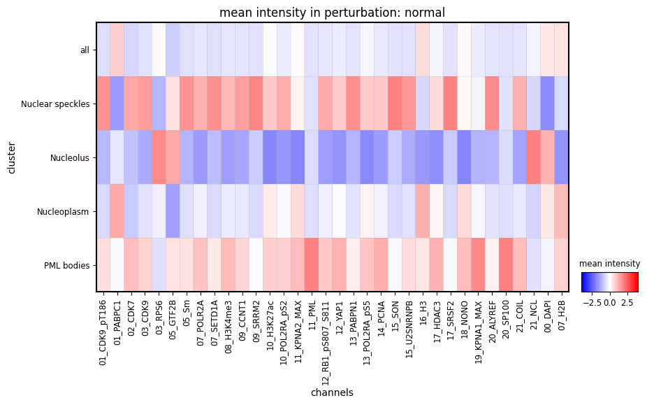
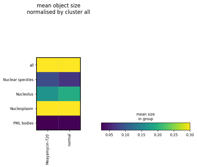
Using this combined adata, we can plot the mean intensity of each channel in each CSL and the size of each CSL in the unperturbed cells using plot_mean_intensity and plot_mean_size

plot_mean_intensity(
    adata_intensity,
    groupby="cluster",
    limit_to_groups={"perturbation": "normal"},
    dendrogram=False,
    layer=None,
    standard_scale="var",
    cmap="bwr",
    vmin=-4,
    vmax=4,
)
plot_mean_size(
    adata_intensity,
    groupby_row="cluster",
    groupby_col="perturbation_duration",
    normby_row="all",
    vmax=0.3,
)

/home/icb/hannah.spitzer/projects/pelkmans/software_new/campa/campa/pl/_intensity_features.py:222: FutureWarning: The default value of numeric_only in DataFrameGroupBy.mean is deprecated. In a future version, numeric_only will default to False. Either specify numeric_only or select only columns which should be valid for the function.
  c: adata[adata.obs[groupby_col] == c].obs.groupby(groupby_row).mean()["size"]
/home/icb/hannah.spitzer/projects/pelkmans/software_new/campa/campa/pl/_intensity_features.py:222: FutureWarning: The default value of numeric_only in DataFrameGroupBy.mean is deprecated. In a future version, numeric_only will default to False. Either specify numeric_only or select only columns which should be valid for the function.
  c: adata[adata.obs[groupby_col] == c].obs.groupby(groupby_row).mean()["size"]

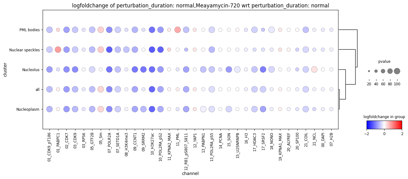
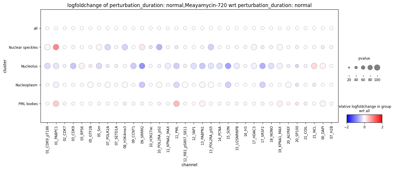
Now, let us visualise the log2fold change in intensity in the Meayamycin perturbation compared to unperturbed cells with plot_intensity_change. This plots a dot plot of clusters by channels. The colour of each dot is the log2fold change in intensity compared to unperturbed cells. The size of the dots indicated the p-value. Small dots are non-significant intensity changes, large dots are significant (p > alpha). For the sake of speed, here, p-values are determined using a t-test, for more accurate p-values, please use pval='mixed_model', which will include well as random effect.

The first plot shows the log2fold change, and the second plot the relative log2fold change per CSL, obtained by dividing the values by the “all” column (norm_by_group='all')

res = get_intensity_change(
    adata_intensity,
    groupby="cluster",
    reference_group="perturbation_duration",
    reference=["normal"],
    limit_to_groups={"perturbation_duration": ["normal", "Meayamycin-720"]},
    color="logfoldchange",
    size="pval",
    pval="ttest",
)
plot_intensity_change(**res, adjust_height=True, figsize=(15, 5), vmin=-2, vmax=2, dendrogram=True)

res = get_intensity_change(
    adata_intensity,
    groupby="cluster",
    reference_group="perturbation_duration",
    reference=["normal"],
    limit_to_groups={"perturbation_duration": ["normal", "Meayamycin-720"]},
    color="logfoldchange",
    size="pval",
    pval="ttest",
    norm_by_group="all",
)
plot_intensity_change(**res, adjust_height=True, figsize=(15, 5), vmin=-2, vmax=2)

WARNING: dendrogram data not found (using key=dendrogram_cluster). Running `sc.tl.dendrogram` with default parameters. For fine tuning it is recommended to run `sc.tl.dendrogram` independently.

/home/icb/hannah.spitzer/miniconda3/envs/campa/lib/python3.9/site-packages/scanpy/plotting/_dotplot.py:749: UserWarning: No data for colormapping provided via 'c'. Parameters 'cmap', 'norm' will be ignored
  dot_ax.scatter(x, y, **kwds)
/home/icb/hannah.spitzer/projects/pelkmans/software_new/campa/campa/pl/_intensity_features.py:459: RuntimeWarning: Precision loss occurred in moment calculation due to catastrophic cancellation. This occurs when the data are nearly identical. Results may be unreliable.
  _, pvals = scipy.stats.ttest_ind(cur_ref_expr, g_expr, axis=0)
/home/icb/hannah.spitzer/miniconda3/envs/campa/lib/python3.9/site-packages/scanpy/plotting/_dotplot.py:749: UserWarning: No data for colormapping provided via 'c'. Parameters 'cmap', 'norm' will be ignored
  dot_ax.scatter(x, y, **kwds)

Co-occurrence scores

Co-occurrence scores are calculated for each cluster-cluster pair. They are stored in adata.obsm['co_occurrence_{cluster1}_{cluster2}'] as a n cells x distances matrix. The distances used can be found in adata.uns['co_occurrence_params'].

extr = extrs[0]
display(extr.adata.obsm["co_occurrence_Nucleolus_Nuclear speckles"])

print(extr.adata.uns["co_occurrence_params"])

	0	1	2	3
0	0.020466	0.129805	0.733902	1.106458
1	0.118672	0.361029	0.867357	1.069965
2	0.062864	0.266752	0.787869	1.159926
3	0.035031	0.120766	0.550169	1.213713
4	0.000458	0.060348	0.623832	1.188438
5	0.000000	0.000000	0.129918	1.871468
6	0.043499	0.271834	0.901377	1.108016
7	0.042482	0.246719	0.788401	1.192697
8	0.000000	0.000000	0.000000	0.000000
9	0.011935	0.181210	1.058228	1.093186
10	0.114000	0.454269	0.865092	1.167536
11	0.019074	0.189035	0.644840	1.052670

{'interval': array([ 2.       ,  4.6806946, 10.954452 , 25.63722  , 60.       ],
      dtype=float32)}

It is possible to export the co-occurrence information in one csv file for each CSL-CSL pair using [FeatureExtractor.extract_co_occurrence_csv][]. The resulting csv file contains the co-occurrence scores for each distance interval as columns and cells as rows, as well as additionally defined columns. This saves one csv file per CSL-CSL pair in experiment_dir/aggregated/full_data/data_dir/export.

for extr in extrs:
    extr.extract_co_occurrence_csv(obs=["well_name", "perturbation_duration", "TR"])

extr = extrs[0]
# check if results are stored
save_dir = os.path.join(os.path.dirname(extr.fname), "export")
print("csv exported to", save_dir)
print([n for n in os.listdir(save_dir) if "co_occurrence" in n])

display(pd.read_csv(os.path.join(save_dir, "co_occurrence_Nucleoplasm_Nucleolus_features_annotation.csv"), index_col=0))

csv exported to /home/icb/hannah.spitzer/projects/pelkmans/software_new/campa_notebooks_test/example_experiments/test_pre_trained/CondVAE_pert-CC/aggregated/full_data/184A1_unperturbed/I09/export
['co_occurrence_PML bodies_Nuclear speckles_features_annotation.csv', 'co_occurrence_Nucleoplasm_Nuclear speckles_features_annotation.csv', 'co_occurrence_Nucleoplasm_Nucleolus_features_annotation.csv', 'co_occurrence_Nucleolus_PML bodies_features_annotation.csv', 'co_occurrence_Nuclear speckles_Nuclear speckles_features_annotation.csv', 'co_occurrence_PML bodies_Nucleolus_features_annotation.csv', 'co_occurrence_PML bodies_Nucleoplasm_features_annotation.csv', 'co_occurrence_Nucleolus_Nucleolus_features_annotation.csv', 'co_occurrence_Nuclear speckles_PML bodies_features_annotation.csv', 'co_occurrence_PML bodies_PML bodies_features_annotation.csv', 'co_occurrence_Nucleoplasm_PML bodies_features_annotation.csv', 'co_occurrence_Nuclear speckles_Nucleoplasm_features_annotation.csv', 'co_occurrence_Nucleolus_Nucleoplasm_features_annotation.csv', 'co_occurrence_Nuclear speckles_Nucleolus_features_annotation.csv', 'co_occurrence_Nucleolus_Nuclear speckles_features_annotation.csv', 'co_occurrence_Nucleoplasm_Nucleoplasm_features_annotation.csv']

	2.00-4.68	4.68-10.95	10.95-25.64	25.64-60.00	mapobject_id	well_name	perturbation_duration	TR
0	0.217142	0.451038	0.831327	1.048945	205776	I09	normal	357.672008
1	0.185153	0.335840	0.631343	1.033807	205790	I09	normal	428.364268
2	0.217809	0.353777	0.604462	1.113828	248082	I09	normal	250.488581
3	0.247925	0.441065	0.739990	1.001092	248102	I09	normal	515.735421
4	0.161814	0.340358	0.684436	1.029913	259784	I09	normal	348.150713
5	0.811214	1.009496	1.028775	0.992664	291041	I09	normal	443.565445
6	0.217856	0.447180	0.789221	1.093390	345908	I09	normal	316.004105
7	0.204482	0.405060	0.791247	1.076277	359378	I09	normal	367.904255
8	0.545410	0.831929	1.024679	1.010255	359393	I09	normal	513.668590
9	0.194497	0.413888	0.750494	1.032792	366493	I09	normal	330.847832
10	0.236510	0.432413	0.801058	1.047899	383341	I09	normal	388.012319
11	0.183172	0.370742	0.700137	1.014940	383793	I09	normal	376.243596

We can plot co-occurrence scores by using plot_co_occurrence or plot_co_occurrence_grid. First, we need to combine all adata objects into one. For this, we can use AnnData.concat.

# get combined adata
adata_co_occ = ad.concat([extr.adata for extr in extrs], index_unique="-", uns_merge="same")

print("co-occurrence scores:", adata_co_occ.obsm)

co-occurrence scores: AxisArrays with keys: co_occurrence_Nuclear speckles_Nuclear speckles, co_occurrence_Nuclear speckles_Nucleolus, co_occurrence_Nuclear speckles_Nucleoplasm, co_occurrence_Nuclear speckles_PML bodies, co_occurrence_Nucleolus_Nuclear speckles, co_occurrence_Nucleolus_Nucleolus, co_occurrence_Nucleolus_Nucleoplasm, co_occurrence_Nucleolus_PML bodies, co_occurrence_Nucleoplasm_Nuclear speckles, co_occurrence_Nucleoplasm_Nucleolus, co_occurrence_Nucleoplasm_Nucleoplasm, co_occurrence_Nucleoplasm_PML bodies, co_occurrence_PML bodies_Nuclear speckles, co_occurrence_PML bodies_Nucleolus, co_occurrence_PML bodies_Nucleoplasm, co_occurrence_PML bodies_PML bodies, size

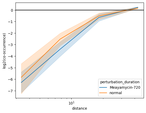
With plot_co_occurrence we can plot one cluster-cluster pair. With condition we can define the grouping of scores. Each group will be displayed by a separate line on the co-occurrence plot.

The co-occurrence plot shows the calculated co-occurrence scores for each distance interval. Here, we show the mean co-occurrence values and their 95th confidence interval obtained through bootstrapping.

# plot meam co-occ scores
condition = "perturbation_duration"
condition_values = None

# for one cluster-cluster pairing
plot_co_occurrence(adata_co_occ, "Nucleolus", "Nuclear speckles", condition, condition_values, ci=95)

/home/icb/hannah.spitzer/projects/pelkmans/software_new/campa/campa/pl/_spatial_features.py:70: FutureWarning:

The `ci` parameter is deprecated. Use `errorbar=('ci', 95)` for the same effect.

  g = sns.lineplot(data=scores, y="score", x="distance", hue=condition, ax=ax, **kwargs)

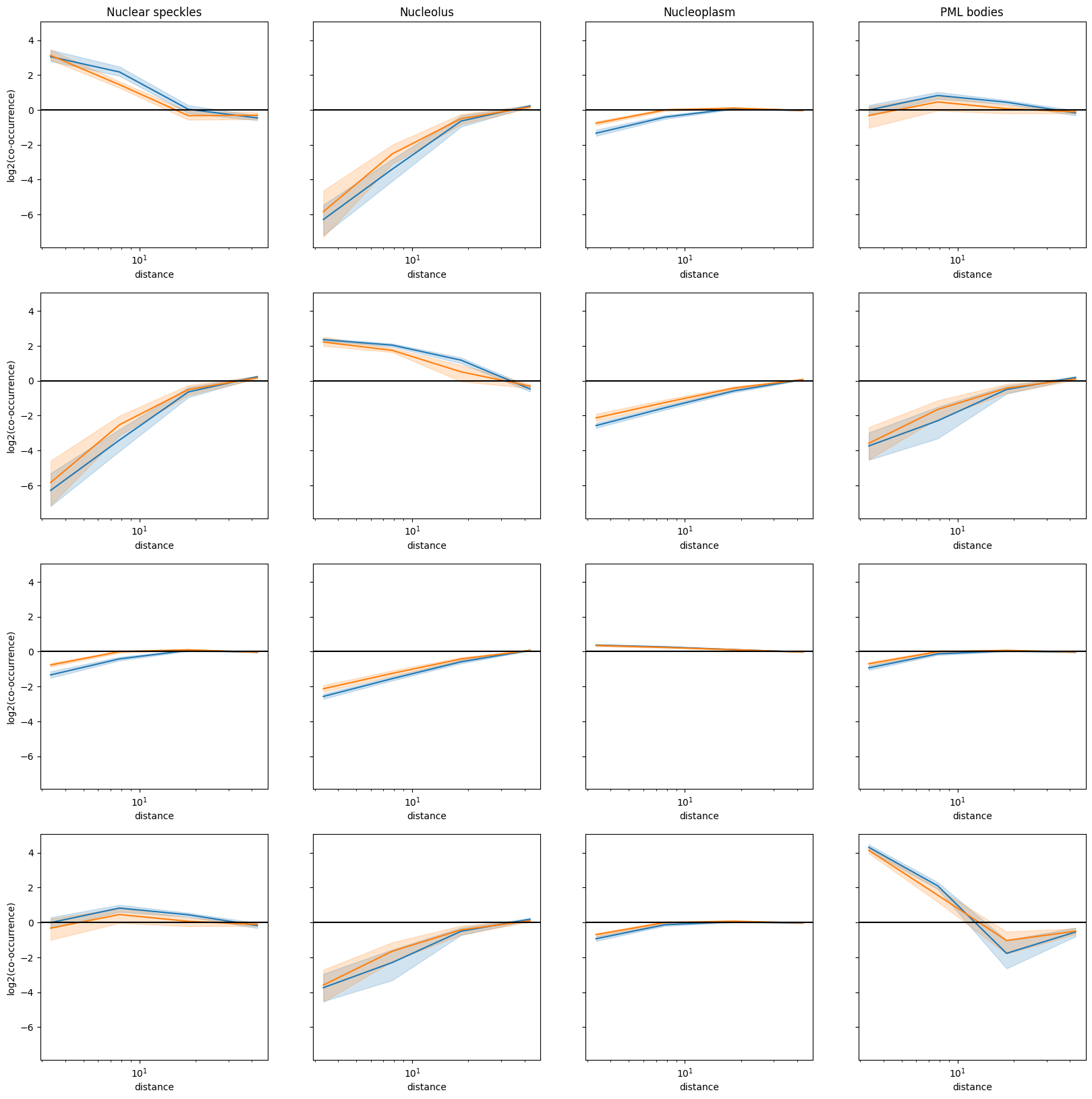
With plot_co_occurrence_grid we can plot an overview of all cluster-cluster pairs.

fig, axes = plot_co_occurrence_grid(adata_co_occ, condition, condition_values, legend=False, ci=95, figsize=(20, 20))

/home/icb/hannah.spitzer/projects/pelkmans/software_new/campa/campa/pl/_spatial_features.py:70: FutureWarning:

The `ci` parameter is deprecated. Use `errorbar=('ci', 95)` for the same effect.

  g = sns.lineplot(data=scores, y="score", x="distance", hue=condition, ax=ax, **kwargs)
/home/icb/hannah.spitzer/projects/pelkmans/software_new/campa/campa/pl/_spatial_features.py:70: FutureWarning:

The `ci` parameter is deprecated. Use `errorbar=('ci', 95)` for the same effect.

  g = sns.lineplot(data=scores, y="score", x="distance", hue=condition, ax=ax, **kwargs)
/home/icb/hannah.spitzer/projects/pelkmans/software_new/campa/campa/pl/_spatial_features.py:70: FutureWarning:

The `ci` parameter is deprecated. Use `errorbar=('ci', 95)` for the same effect.

  g = sns.lineplot(data=scores, y="score", x="distance", hue=condition, ax=ax, **kwargs)
/home/icb/hannah.spitzer/projects/pelkmans/software_new/campa/campa/pl/_spatial_features.py:70: FutureWarning:

The `ci` parameter is deprecated. Use `errorbar=('ci', 95)` for the same effect.

  g = sns.lineplot(data=scores, y="score", x="distance", hue=condition, ax=ax, **kwargs)
/home/icb/hannah.spitzer/projects/pelkmans/software_new/campa/campa/pl/_spatial_features.py:70: FutureWarning:

The `ci` parameter is deprecated. Use `errorbar=('ci', 95)` for the same effect.

  g = sns.lineplot(data=scores, y="score", x="distance", hue=condition, ax=ax, **kwargs)
/home/icb/hannah.spitzer/projects/pelkmans/software_new/campa/campa/pl/_spatial_features.py:70: FutureWarning:

The `ci` parameter is deprecated. Use `errorbar=('ci', 95)` for the same effect.

  g = sns.lineplot(data=scores, y="score", x="distance", hue=condition, ax=ax, **kwargs)
/home/icb/hannah.spitzer/projects/pelkmans/software_new/campa/campa/pl/_spatial_features.py:70: FutureWarning:

The `ci` parameter is deprecated. Use `errorbar=('ci', 95)` for the same effect.

  g = sns.lineplot(data=scores, y="score", x="distance", hue=condition, ax=ax, **kwargs)
/home/icb/hannah.spitzer/projects/pelkmans/software_new/campa/campa/pl/_spatial_features.py:70: FutureWarning:

The `ci` parameter is deprecated. Use `errorbar=('ci', 95)` for the same effect.

  g = sns.lineplot(data=scores, y="score", x="distance", hue=condition, ax=ax, **kwargs)
/home/icb/hannah.spitzer/projects/pelkmans/software_new/campa/campa/pl/_spatial_features.py:70: FutureWarning:

The `ci` parameter is deprecated. Use `errorbar=('ci', 95)` for the same effect.

  g = sns.lineplot(data=scores, y="score", x="distance", hue=condition, ax=ax, **kwargs)
/home/icb/hannah.spitzer/projects/pelkmans/software_new/campa/campa/pl/_spatial_features.py:70: FutureWarning:

The `ci` parameter is deprecated. Use `errorbar=('ci', 95)` for the same effect.

  g = sns.lineplot(data=scores, y="score", x="distance", hue=condition, ax=ax, **kwargs)
/home/icb/hannah.spitzer/projects/pelkmans/software_new/campa/campa/pl/_spatial_features.py:70: FutureWarning:

The `ci` parameter is deprecated. Use `errorbar=('ci', 95)` for the same effect.

  g = sns.lineplot(data=scores, y="score", x="distance", hue=condition, ax=ax, **kwargs)
/home/icb/hannah.spitzer/projects/pelkmans/software_new/campa/campa/pl/_spatial_features.py:70: FutureWarning:

The `ci` parameter is deprecated. Use `errorbar=('ci', 95)` for the same effect.

  g = sns.lineplot(data=scores, y="score", x="distance", hue=condition, ax=ax, **kwargs)
/home/icb/hannah.spitzer/projects/pelkmans/software_new/campa/campa/pl/_spatial_features.py:70: FutureWarning:

The `ci` parameter is deprecated. Use `errorbar=('ci', 95)` for the same effect.

  g = sns.lineplot(data=scores, y="score", x="distance", hue=condition, ax=ax, **kwargs)
/home/icb/hannah.spitzer/projects/pelkmans/software_new/campa/campa/pl/_spatial_features.py:70: FutureWarning:

The `ci` parameter is deprecated. Use `errorbar=('ci', 95)` for the same effect.

  g = sns.lineplot(data=scores, y="score", x="distance", hue=condition, ax=ax, **kwargs)
/home/icb/hannah.spitzer/projects/pelkmans/software_new/campa/campa/pl/_spatial_features.py:70: FutureWarning:

The `ci` parameter is deprecated. Use `errorbar=('ci', 95)` for the same effect.

  g = sns.lineplot(data=scores, y="score", x="distance", hue=condition, ax=ax, **kwargs)
/home/icb/hannah.spitzer/projects/pelkmans/software_new/campa/campa/pl/_spatial_features.py:70: FutureWarning:

The `ci` parameter is deprecated. Use `errorbar=('ci', 95)` for the same effect.

  g = sns.lineplot(data=scores, y="score", x="distance", hue=condition, ax=ax, **kwargs)

Object statistics

Object statistics are features extracted from connected components per cluster for each cell. Possible features are area, circlularity, elongation, and extent of connected components. Per component/region features are calculated and stored in adata.uns['object_stats'].

display(extrs[0].adata.uns["object_stats"])

	area	circularity	elongation	extent	mapobject_id	clustering
0	9045	0.043528	0.227821	0.471585	205776	Nucleoplasm
1	978	0.638093	0.116856	0.735338	205776	Nucleolus
2	29	1.000000	0.096517	0.805556	205776	Nucleolus
3	256	0.541414	0.534975	0.561404	205776	Nuclear speckles
4	38	1.000000	0.321553	0.791667	205776	PML bodies
...	...	...	...	...	...	...
346	98	0.810891	0.307977	0.753846	383793	Nuclear speckles
347	125	0.906486	0.290123	0.694444	383793	Nuclear speckles
348	14	1.000000	0.249786	0.700000	383793	Nuclear speckles
349	17	0.936106	0.524493	0.472222	383793	PML bodies
350	54	0.974758	0.269712	0.600000	383793	PML bodies

351 rows × 6 columns

To aggregate this information to per-cell level, FeatureExtractor.get_object_stats is used. This aggregated the data with the provided aggregation function and stores the result in adata.obsm['object_stats_agg']. In addition, we can filter small areas below area_threshold prior to aggregation.

# aggregate object statistics using median
for extr in extrs:
    _ = extr.get_object_stats(area_threshold=10, agg=["median"])

# combined adatas for plotting
adata_object_stats = ad.concat([extr.adata for extr in extrs], index_unique="-", uns_merge="same")

adata_object_stats contains aggregated per cell object stats in obsm:

adata_object_stats.obsm["object_stats_agg"]

	area_median|Nuclear speckles	area_median|Nucleolus	area_median|Nucleoplasm	area_median|PML bodies	circularity_median|Nuclear speckles	circularity_median|Nucleolus	circularity_median|Nucleoplasm	circularity_median|PML bodies	elongation_median|Nuclear speckles	elongation_median|Nucleolus	elongation_median|Nucleoplasm	elongation_median|PML bodies	extent_median|Nuclear speckles	extent_median|Nucleolus	extent_median|Nucleoplasm	extent_median|PML bodies	count|Nuclear speckles	count|Nucleolus	count|Nucleoplasm	count|PML bodies
0-0	87.0	978.0	9045.0	42.5	0.861312	0.638093	0.043528	1.000000	0.285864	0.116856	0.227821	0.310047	0.633333	0.735338	0.471585	0.742063	11.0	3.0	1.0	6.0
1-0	97.5	438.0	9457.0	49.0	0.732411	0.411849	0.036234	0.959830	0.412936	0.337495	0.354512	0.253441	0.617695	0.551043	0.426221	0.711111	12.0	3.0	1.0	7.0
2-0	89.0	2365.0	4194.5	76.0	0.834565	0.131215	0.236317	0.957019	0.222408	0.349102	0.403929	0.199730	0.662551	0.532658	0.375361	0.714583	10.0	1.0	2.0	12.0
3-0	42.0	2593.0	13.0	36.0	0.863145	0.094925	1.000000	1.000000	0.355378	0.203823	0.307020	0.175429	0.607143	0.449004	0.501330	0.759736	9.0	1.0	3.0	12.0
4-0	72.0	1157.0	15376.0	57.0	0.905092	0.381709	0.040231	1.000000	0.381959	0.233705	0.330665	0.175379	0.610185	0.600415	0.513355	0.777778	16.0	3.0	1.0	9.0
5-0	32.0	18.0	6580.0	97.5	1.000000	1.000000	0.297695	0.858740	0.068028	0.226034	0.343594	0.125506	0.761905	0.666667	0.679051	0.799632	1.0	2.0	1.0	2.0
6-0	66.0	959.0	7758.0	27.0	0.961701	0.432387	0.051205	1.000000	0.244032	0.460579	0.261960	0.190607	0.716852	0.549069	0.502331	0.771429	14.0	2.0	1.0	6.0
7-0	65.0	1055.5	7234.0	38.0	0.885201	0.598381	0.054602	1.000000	0.366449	0.562931	0.310322	0.117958	0.635417	0.445033	0.502780	0.727273	11.0	2.0	1.0	5.0
8-0	0.0	78.0	8453.0	82.5	0.000000	0.512022	0.147361	0.884891	0.000000	0.290167	0.271034	0.148813	0.000000	0.537500	0.635659	0.675196	0.0	3.0	1.0	2.0
9-0	72.0	1444.5	10587.0	63.0	0.853768	0.380567	0.052200	0.993804	0.405150	0.681782	0.234737	0.123254	0.600000	0.510217	0.542367	0.750000	11.0	2.0	1.0	5.0
10-0	39.0	1043.0	7398.0	58.5	0.932875	0.436683	0.048323	1.000000	0.388201	0.458571	0.185267	0.236344	0.571429	0.477905	0.556324	0.738112	13.0	2.0	1.0	6.0
11-0	98.0	2805.0	8993.0	41.0	0.845314	0.239826	0.043590	0.988189	0.307977	0.211277	0.140934	0.336398	0.695378	0.572449	0.498062	0.696429	11.0	1.0	1.0	9.0
0-1	33.0	646.0	8387.0	90.0	0.984769	0.475397	0.056057	0.933442	0.402862	0.338597	0.085823	0.272680	0.565657	0.630244	0.541796	0.752778	7.0	3.0	1.0	2.0
1-1	40.0	4164.0	13403.0	41.0	1.000000	0.173680	0.036768	1.000000	0.376558	0.306077	0.159526	0.068881	0.641327	0.484186	0.510882	0.765152	20.0	1.0	1.0	10.0
2-1	88.0	1151.0	8304.0	23.0	0.742052	0.106195	0.064869	1.000000	0.315780	0.619785	0.103333	0.146457	0.599495	0.414924	0.572690	0.666667	8.0	1.0	1.0	9.0
3-1	64.0	2252.0	7856.0	43.0	0.857538	0.173152	0.059856	1.000000	0.267228	0.202500	0.245970	0.137212	0.653061	0.446825	0.508282	0.760000	9.0	1.0	1.0	7.0
4-1	91.0	2868.0	7387.0	51.0	0.756498	0.221948	0.035140	1.000000	0.312715	0.171164	0.349126	0.112509	0.606981	0.510684	0.467295	0.741667	10.0	1.0	1.0	6.0
5-1	31.0	1652.0	9770.0	47.0	0.689846	0.241960	0.050961	1.000000	0.211355	0.277617	0.288946	0.253809	0.574074	0.494759	0.549278	0.763788	5.0	1.0	1.0	6.0
6-1	57.0	873.0	22.0	27.0	0.863797	0.158189	0.751116	1.000000	0.337476	0.424378	0.370224	0.182968	0.631944	0.467984	0.418750	0.750000	9.0	2.0	4.0	8.0
7-1	54.0	659.0	6997.0	26.0	0.856820	0.465333	0.074767	1.000000	0.441801	0.482696	0.220509	0.162121	0.604167	0.591435	0.538396	0.722222	5.0	3.0	1.0	3.0
8-1	68.0	1110.5	8052.0	49.5	0.848859	0.808536	0.096679	1.000000	0.295531	0.124259	0.340513	0.243407	0.656250	0.757819	0.515559	0.756818	5.0	2.0	1.0	6.0
9-1	126.0	584.0	5990.0	57.5	0.752271	0.233462	0.068063	1.000000	0.353340	0.384750	0.112466	0.169162	0.641026	0.565739	0.548836	0.692956	5.0	2.0	1.0	4.0
10-1	77.5	48.0	12283.0	58.0	0.832699	0.389967	0.035018	1.000000	0.331494	0.679027	0.271263	0.087320	0.600069	0.325420	0.515464	0.714286	10.0	6.0	1.0	9.0
11-1	24.0	1602.0	12253.0	36.5	0.871560	0.371284	0.063537	1.000000	0.317529	0.486609	0.322754	0.254069	0.510204	0.526215	0.580024	0.722222	7.0	2.0	1.0	8.0
12-1	82.0	2723.0	8338.0	60.0	0.901766	0.418904	0.058905	1.000000	0.311033	0.392981	0.317050	0.219982	0.656250	0.702528	0.486891	0.732143	9.0	1.0	1.0	7.0
13-1	59.0	3417.0	10921.0	39.5	0.875924	0.156722	0.046924	1.000000	0.284057	0.460068	0.246043	0.162387	0.589927	0.483173	0.512867	0.755102	12.0	1.0	1.0	4.0
0-2	81.0	506.0	6095.0	59.5	0.874082	0.692071	0.061450	0.813102	0.271903	0.204649	0.566809	0.318936	0.640152	0.709939	0.376095	0.680556	6.0	3.0	1.0	2.0
1-2	112.0	1028.0	18268.0	47.0	0.684060	0.651009	0.057497	1.000000	0.461039	0.224796	0.272422	0.176686	0.534722	0.668787	0.555934	0.750000	9.0	3.0	1.0	11.0
2-2	158.0	2256.0	11749.0	58.0	0.772462	0.298946	0.072532	1.000000	0.262487	0.553125	0.176129	0.160893	0.670455	0.502674	0.568821	0.805556	7.0	1.0	1.0	7.0
3-2	231.5	2455.0	9577.0	50.0	0.704407	0.394730	0.070778	1.000000	0.377610	0.272570	0.451540	0.159108	0.657225	0.631430	0.454878	0.691358	6.0	1.0	1.0	5.0
4-2	151.0	3289.0	11322.0	40.0	0.767014	0.349287	0.048491	1.000000	0.311007	0.651149	0.319685	0.172907	0.633250	0.413399	0.471691	0.714286	12.0	1.0	1.0	7.0
5-2	205.5	16.0	11118.0	21.0	0.662480	1.000000	0.086700	1.000000	0.447544	0.193111	0.178973	0.181705	0.624603	0.601638	0.580514	0.718182	4.0	3.0	1.0	14.0
6-2	39.0	4629.0	18873.0	66.0	0.882109	0.277760	0.062439	1.000000	0.279717	0.502306	0.069330	0.102909	0.638826	0.495345	0.577209	0.738905	8.0	1.0	1.0	8.0
7-2	424.5	937.5	10973.0	73.5	0.552564	0.664226	0.079359	0.957464	0.440302	0.258909	0.249811	0.271398	0.596174	0.643831	0.513910	0.668182	4.0	2.0	1.0	8.0
8-2	86.0	1448.0	12608.0	80.0	0.748017	0.390063	0.051236	0.974549	0.345564	0.475289	0.208464	0.180974	0.547619	0.588658	0.555125	0.688312	11.0	2.0	1.0	5.0
9-2	109.0	2110.0	8335.0	47.0	0.819828	0.562741	0.081130	0.950839	0.330001	0.478976	0.084208	0.354715	0.644192	0.793233	0.521851	0.679457	6.0	1.0	1.0	4.0
10-2	76.0	2238.0	12062.0	37.0	0.715299	0.618056	0.077079	1.000000	0.481178	0.283293	0.247034	0.130520	0.633971	0.744016	0.574709	0.750000	8.0	1.0	1.0	9.0
0-3	26.0	38.5	10357.0	70.5	0.715492	0.848255	0.073592	0.955768	0.555150	0.312634	0.151869	0.268488	0.496795	0.592727	0.543047	0.671364	7.0	4.0	1.0	6.0
1-3	159.0	1142.0	8944.0	76.0	0.823861	0.261123	0.058375	0.995851	0.194221	0.462433	0.130762	0.143551	0.672059	0.454495	0.507951	0.773810	8.0	2.0	1.0	5.0
2-3	193.0	450.0	9745.0	34.0	0.802449	0.489826	0.052970	0.995891	0.389129	0.206004	0.216125	0.355088	0.642857	0.573980	0.541389	0.686012	7.0	3.0	1.0	8.0
3-3	130.0	780.0	15704.0	66.0	0.617096	0.618706	0.038042	0.990273	0.371340	0.227953	0.140536	0.143821	0.669643	0.633333	0.523991	0.686065	11.0	5.0	1.0	10.0
4-3	0.0	177.0	12530.0	25.5	0.000000	0.588240	0.092439	1.000000	0.000000	0.315782	0.190005	0.255248	0.000000	0.650735	0.617972	0.600446	0.0	3.0	1.0	6.0
5-3	115.5	726.0	12691.0	78.0	0.813633	0.541090	0.056721	0.915472	0.306740	0.242757	0.298018	0.127670	0.662764	0.583153	0.511322	0.702040	10.0	4.0	1.0	6.0
6-3	337.0	1795.0	12922.0	75.0	0.605931	0.522038	0.058115	0.946450	0.430918	0.306800	0.101516	0.095062	0.540936	0.620238	0.524432	0.705128	5.0	2.0	1.0	11.0
7-3	164.0	1272.5	18073.0	47.0	0.685409	0.676682	0.042065	1.000000	0.373616	0.197385	0.228095	0.141581	0.622322	0.655476	0.515988	0.750000	12.0	4.0	1.0	9.0
8-3	154.5	3365.0	13819.0	52.0	0.788247	0.321839	0.062378	1.000000	0.260891	0.695200	0.194789	0.192065	0.697316	0.449866	0.532073	0.757716	8.0	1.0	1.0	6.0

It is possible to export the object stats in a csv file using FeatureExtractor.extract_object_stats_csv. The resulting csv file contains the aggregated object stats matrix from adata_object_stats.obsm['object_stats_agg'] as well as additionally defined columns. This saves one csv file per CSL-CSL pair in experiment_dir/aggregated/full_data/data_dir/export.

for extr in extrs:
    extr.extract_object_stats_csv(obs=["well_name", "perturbation_duration", "TR"])

extr = extrs[0]
# check if results are stored
save_dir = os.path.join(os.path.dirname(extr.fname), "export")
print("csv exported to", save_dir)
print([n for n in os.listdir(save_dir) if "object_stats" in n])

csv exported to /home/icb/hannah.spitzer/projects/pelkmans/software_new/campa_notebooks_test/example_experiments/test_pre_trained/CondVAE_pert-CC/aggregated/full_data/184A1_unperturbed/I09/export
['object_stats_features_annotation.csv']

plot_object_stats can be used to plot a box-plot overview of the object stats. Again, we can define the grouping using group_key.

plot_object_stats(adata_object_stats, group_key="perturbation_duration", figsize_mult=(4, 4))