Cluster data into CSLs

Using the trained condVAE_pert-CC model, this tutorial looks at how to cluster the learned latent representation into CSLs. In order to ensure that the clusters and their annotations are reproducible, we will use a pretrained model in this example. You can also use the model that you trained in the Train and evaluate models tutorial, but due to the randomness of training neural networks, the latent space might be different, resulting in different clusters.

In this tutorial we will:

create and cluster a smaller subset of the large dataset
interactively cluster the data
query the Human Protein Atlas to get candidate annotations
annotate the data and plot the results on example cells
prepare the entire dataset for clustering
project the clustering to the entire dataset

[1]:

from pathlib import Path
import os

from IPython.display import display
import numpy as np
import pandas as pd
import scanpy as sc
import seaborn as sns
import matplotlib.pyplot as plt

from campa.pl import annotate_img
from campa.tl import (
    Cluster,
    Experiment,
    create_cluster_data,
    get_clustered_cells,
    load_full_data_dict,
    prepare_full_dataset,
    project_cluster_data,
    add_clustering_to_adata,
)
from campa.data import MPPData, load_example_data, load_example_experiment
from campa.utils import init_logging
from campa.constants import campa_config

# init logging with level INFO=20, WARNING=30
init_logging(level=30)
# ensure that example data is downloaded
load_example_data()
# read correct campa_config -- created with setup.ipynb
CAMPA_DIR = Path.cwd()
campa_config.config_fname = CAMPA_DIR / "params/campa.ini"
print(campa_config)

2022-11-25 11:51:22.297858: I tensorflow/core/platform/cpu_feature_guard.cc:193] This TensorFlow binary is optimized with oneAPI Deep Neural Network Library (oneDNN) to use the following CPU instructions in performance-critical operations:  AVX2 AVX512F AVX512_VNNI FMA
To enable them in other operations, rebuild TensorFlow with the appropriate compiler flags.
2022-11-25 11:51:22.485116: I tensorflow/core/util/util.cc:169] oneDNN custom operations are on. You may see slightly different numerical results due to floating-point round-off errors from different computation orders. To turn them off, set the environment variable `TF_ENABLE_ONEDNN_OPTS=0`.
2022-11-25 11:51:22.529442: E tensorflow/stream_executor/cuda/cuda_blas.cc:2981] Unable to register cuBLAS factory: Attempting to register factory for plugin cuBLAS when one has already been registered

Reading config from /home/icb/hannah.spitzer/projects/pelkmans/software_new/campa_notebooks_test/params/campa.ini
CAMPAConfig (fname: /home/icb/hannah.spitzer/projects/pelkmans/software_new/campa_notebooks_test/params/campa.ini)
EXPERIMENT_DIR: /home/icb/hannah.spitzer/projects/pelkmans/software_new/campa_notebooks_test/example_experiments
BASE_DATA_DIR: /home/icb/hannah.spitzer/projects/pelkmans/software_new/campa_notebooks_test/example_data
CO_OCC_CHUNK_SIZE: 10000000.0
data_config/exampledata: /home/icb/hannah.spitzer/projects/pelkmans/software_new/campa_notebooks_test/params/ExampleData_constants.py

First, we need to download the pretrained model

[2]:

example_experiment_folder = load_example_experiment(campa_config.EXPERIMENT_DIR)
print("Example experiment downloaded to:", example_experiment_folder)

Example experiment downloaded to: /home/icb/hannah.spitzer/projects/pelkmans/software_new/campa_notebooks_test/example_experiments/test_pre_trained

Prepare a subset of the data

First, the the data is subsampled, because we would like the clustering to be interactive and feasible to compute on a laptop. If you have more time or access to GPUs, you could also consider to skip the subsampling step and cluster all data directly.

Sub-setting and clustering the data can be done with the high-level API, using create_cluster_data. Alternatively, the CLI can be used:

cd CAMPA_DIR/params
campa cluster test/CondVAE_pert-CC create --subsample --frac 0.1 --save-dir aggregated/sub-0.1 --cluster

If you would like to also directly cluster the data, use cluster=True in the call to create_cluster_data. Here, we leave the clustering for the interactive clustering and annotation step below.

[3]:

create_cluster_data("test_pre_trained/CondVAE_pert-CC", subsample=True, frac=0.1, save_dir="aggregated/sub-0.1")

WARNING:Cluster:Could not load MPPData from test_pre_trained/CondVAE_pert-CC/aggregated/sub-0.1
WARNING:Cluster:Could not load MPPData from test_pre_trained/CondVAE_pert-CC/aggregated/sub-0.1
2022-11-25 11:51:35.375731: I tensorflow/core/platform/cpu_feature_guard.cc:193] This TensorFlow binary is optimized with oneAPI Deep Neural Network Library (oneDNN) to use the following CPU instructions in performance-critical operations:  AVX2 AVX512F AVX512_VNNI FMA
To enable them in other operations, rebuild TensorFlow with the appropriate compiler flags.
2022-11-25 11:51:35.990505: I tensorflow/core/common_runtime/gpu/gpu_device.cc:1616] Created device /job:localhost/replica:0/task:0/device:GPU:0 with 30975 MB memory:  -> device: 0, name: Tesla V100S-PCIE-32GB, pci bus id: 0000:37:00.0, compute capability: 7.0
2022-11-25 11:51:37.894959: I tensorflow/stream_executor/cuda/cuda_dnn.cc:384] Loaded cuDNN version 8202

525/525 [==============================] - 2s 1ms/step

WARNING:MPPData:Saving partial keys of mpp data without a base_data_dir to enable correct loading
/home/icb/hannah.spitzer/miniconda3/envs/campa/lib/python3.9/site-packages/tqdm/auto.py:22: TqdmWarning: IProgress not found. Please update jupyter and ipywidgets. See https://ipywidgets.readthedocs.io/en/stable/user_install.html
  from .autonotebook import tqdm as notebook_tqdm
WARNING:MPPData:Saving partial keys of mpp data without a base_data_dir to enable correct loading

This has created a subset of 10% of all pixels in aggregated/sub-0.1. This again is readable as MPPData. Note that in order to correctly load the MPPData here, we have to define the data_config, and set the base_dir to the EXPERIMENT_DIR, as per default, MPPData looks for data relative to DATA_DIR defined in data_config.

[4]:

cluster_data_dir = "test_pre_trained/CondVAE_pert-CC/aggregated/sub-0.1"
print(os.listdir(os.path.join(campa_config.EXPERIMENT_DIR, cluster_data_dir)))
print(MPPData.from_data_dir(cluster_data_dir, data_config="ExampleData", base_dir=campa_config.EXPERIMENT_DIR))

['channels.csv', 'labels.npy', 'latent.npy', 'y.npy', 'conditions.npy', 'umap.npy', 'mpp.npy', 'obj_ids.npy', 'cluster_params.json', 'metadata.csv', 'x.npy']
MPPData for ExampleData (67084 mpps with shape (3, 3, 34) from 46 objects). Data keys: ['obj_ids', 'x', 'y', 'mpp', 'labels', 'latent', 'conditions'].

Prepare full dataset for projecting cluster to it

To project the clustering to the entire dataset, the model needs to be used to predict the latent representation on all data. It is recommended to run this step in a script, as this might take a while for large datasets:

cd CAMPA_DIR/params
campa cluster test/CondVAE_pert-CC prepare-full --save-dir aggregated/full_data

This script uses the prepare_full_dataset function of the high-level API.

[5]:

prepare_full_dataset("test_pre_trained/CondVAE_pert-CC", save_dir="aggregated/full_data")

iterating over data dirs ['184A1_unperturbed/I09', '184A1_unperturbed/I11', '184A1_meayamycin/I12', '184A1_meayamycin/I20']
1201/1201 [==============================] - 1s 1ms/step
1373/1373 [==============================] - 2s 1ms/step
1412/1412 [==============================] - 2s 1ms/step
1257/1257 [==============================] - 1s 1ms/step

This saves the predicted data to aggregated/full_data. As usual, this can be loaded using MPPData.

[6]:

full_data_dir = "test_pre_trained/CondVAE_pert-CC/aggregated/full_data"
print(os.listdir(os.path.join(campa_config.EXPERIMENT_DIR, full_data_dir)))
# load MPPData from one data_dir
print(
    MPPData.from_data_dir(
        os.path.join(full_data_dir, "184A1_unperturbed/I09"),
        data_config="ExampleData",
        base_dir=campa_config.EXPERIMENT_DIR,
    )
)

['184A1_unperturbed', '184A1_meayamycin']
MPPData for ExampleData (153669 mpps with shape (1, 1, 35) from 12 objects). Data keys: ['obj_ids', 'x', 'y', 'mpp', 'labels', 'latent'].

Interactive clustering and annotation

Now we can cluster our data. This is done by getting an anndata object from the Cluster.cluster_mpp object using MPPData.get_adata and clustering it using scanpy.

Note that for reproducing the clustering we will use the downloaded subsampled and projected data in aggregated/sub-pre for the clustering.

[7]:

# load cl
cluster_data_dir = "test_pre_trained/CondVAE_pert-CC/aggregated/sub-pre"
cl = Cluster.from_cluster_data_dir(cluster_data_dir)
# get adata object
adata = cl.cluster_mpp.get_adata(X="mpp", obsm={"X_latent": "latent", "X_umap": "umap"})

adata contains pixels as obs and protein channels as var. The cVAE latent space is stored in obsm['X_latent'].

[8]:

print("obs:", adata.obs.index)
print("var:", adata.var.index)
print("X_latent shape:", adata.obsm["X_latent"].shape)

obs: Index(['0', '1', '2', '3', '4', '5', '6', '7', '8', '9',
       ...
       '67074', '67075', '67076', '67077', '67078', '67079', '67080', '67081',
       '67082', '67083'],
      dtype='object', length=67084)
var: Index(['01_CDK9_pT186', '01_PABPC1', '02_CDK7', '03_CDK9', '03_RPS6',
       '05_GTF2B', '05_Sm', '07_POLR2A', '07_SETD1A', '08_H3K4me3', '09_CCNT1',
       '09_SRRM2', '10_H3K27ac', '10_POL2RA_pS2', '11_KPNA2_MAX', '11_PML',
       '12_RB1_pS807_S811', '12_YAP1', '13_PABPN1', '13_POL2RA_pS5', '14_PCNA',
       '15_SON', '15_U2SNRNPB', '16_H3', '17_HDAC3', '17_SRSF2', '18_NONO',
       '19_KPNA1_MAX', '20_ALYREF', '20_SP100', '21_COIL', '21_NCL', '00_DAPI',
       '07_H2B'],
      dtype='object', name='name')
X_latent shape: (67084, 16)

Cluster the latent space. Here, different clusterings with different resolutions could be created and compared.

[9]:

# cluster the latent space
sc.pp.neighbors(adata, use_rep="X_latent")
sc.tl.leiden(adata, resolution=0.2, key_added="clustering_res0.2", random_state=0)

[10]:

# write clustering to disk
np.save(
    os.path.join(campa_config.EXPERIMENT_DIR, cluster_data_dir, "clustering_res0.2"), adata.obs["clustering_res0.2"]
)

Explore clustered data

The aim of this step is to annotate the clustering, to aid interpretability of the results. Hereby, CSLs corresponding to the same biological structure may be merged to the same annotated CSL. This annotation is done in an iterative fashion and considers the following factors:

Presence of canonical organelle markers among top enriched channels in each CSL in unperturbed (control) cells. If no canonical markers are present, consider CSL as ‘background’ (i.e. nucleoplasm / cytoplasm).
Spatial distribution of CSLs compared to spatial distribution of canonical markers of organelles in unperturbed (control) cells
Human Protein Atlas subcellular localisation (The Human Protein Atlas, Thul et al. 2017) of top enriched channels in each CSL, weighted by z-scored channel intensity.

Below, we show how to visualise and analyse the clusters for each of these aspects.

Load the Cluster object, and export the Cluster.cluster_mpp with MPPData.get_adata and add the just created clustering to the exported adata object with add_clustering_to_adata.

[11]:

# load cl
cluster_data_dir = "test_pre_trained/CondVAE_pert-CC/aggregated/sub-pre"
cl = Cluster.from_cluster_data_dir(cluster_data_dir)
# get adata object
adata = cl.cluster_mpp.get_adata(X="mpp", obsm={"X_latent": "latent", "X_umap": "umap"})
# add clustering and colormap (from cluster_name_annotation.csv) to adata
cl.set_cluster_name("clustering_res0.2")
add_clustering_to_adata(
    os.path.join(campa_config.EXPERIMENT_DIR, cluster_data_dir), "clustering_res0.2", adata, cl.cluster_annotation
)

Cannot read with memmap:  /home/icb/hannah.spitzer/projects/pelkmans/software_new/campa_notebooks_test/example_experiments/test_pre_trained/CondVAE_pert-CC/aggregated/sub-pre/clustering_res0.2.npy

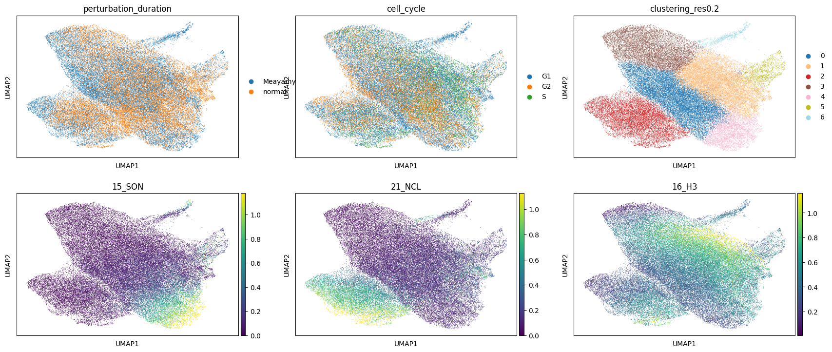
The following is a UMAP of the latent space coordinates of each pixel. It is useful to check that the clustering algorithm is doing something sensible, and also that the conditions used in the autoencoder don’t end up in different regions of the latent space UMAP (which would indicate that the conditional autoencoder was not able to generate a condition-independent representation). Channel intensities can also be visualised here, which is useful if you have some markers for known structures (e.g. NCL, H3, SON)

[12]:

plt.rcParams["figure.figsize"] = [6, 4]
sc.pl.umap(
    adata,
    color=["perturbation_duration", "cell_cycle", "clustering_res0.2", "15_SON", "21_NCL", "16_H3"],
    vmax="p99",
    ncols=3,
)

/home/icb/hannah.spitzer/miniconda3/envs/campa/lib/python3.9/site-packages/scanpy/plotting/_tools/scatterplots.py:392: UserWarning: No data for colormapping provided via 'c'. Parameters 'cmap' will be ignored
  cax = scatter(
/home/icb/hannah.spitzer/miniconda3/envs/campa/lib/python3.9/site-packages/scanpy/plotting/_tools/scatterplots.py:392: UserWarning: No data for colormapping provided via 'c'. Parameters 'cmap' will be ignored
  cax = scatter(
/home/icb/hannah.spitzer/miniconda3/envs/campa/lib/python3.9/site-packages/scanpy/plotting/_tools/scatterplots.py:392: UserWarning: No data for colormapping provided via 'c'. Parameters 'cmap' will be ignored
  cax = scatter(

To begin to understand the identity of each of the clusters, it can be helpful to visualise how the intensity of each of the channels distributes across the clusters:

[13]:

cluster_name = "clustering_res0.2"
pixel_values_annotated = pd.concat(
    [
        pd.DataFrame(adata.X, columns=adata.var_names).reset_index(drop=True),
        adata.obs[[cluster_name]].reset_index(drop=True),
    ],
    axis=1,
)
_ = sns.clustermap(
    pixel_values_annotated.groupby(cluster_name).aggregate("mean"),
    z_score=1,
    cmap="vlag",
    figsize=[14, 9],
    vmin=-3,
    vmax=3,
    method="ward",
)

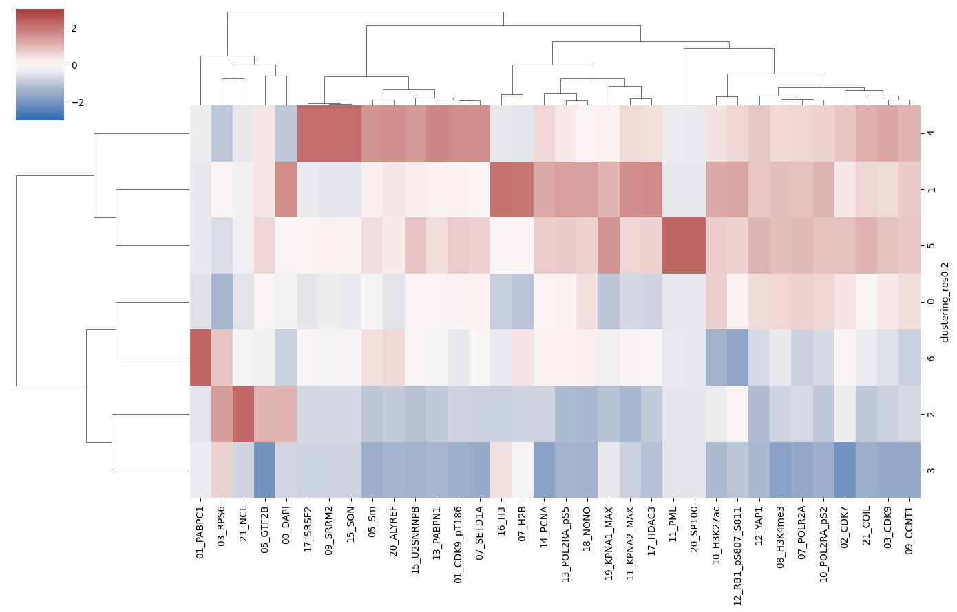
For example, the plot above reveals that PML-body markers PML and SP100 exclusively localise to cluster 5, which is therefore very likely to correspond to PML bodies.

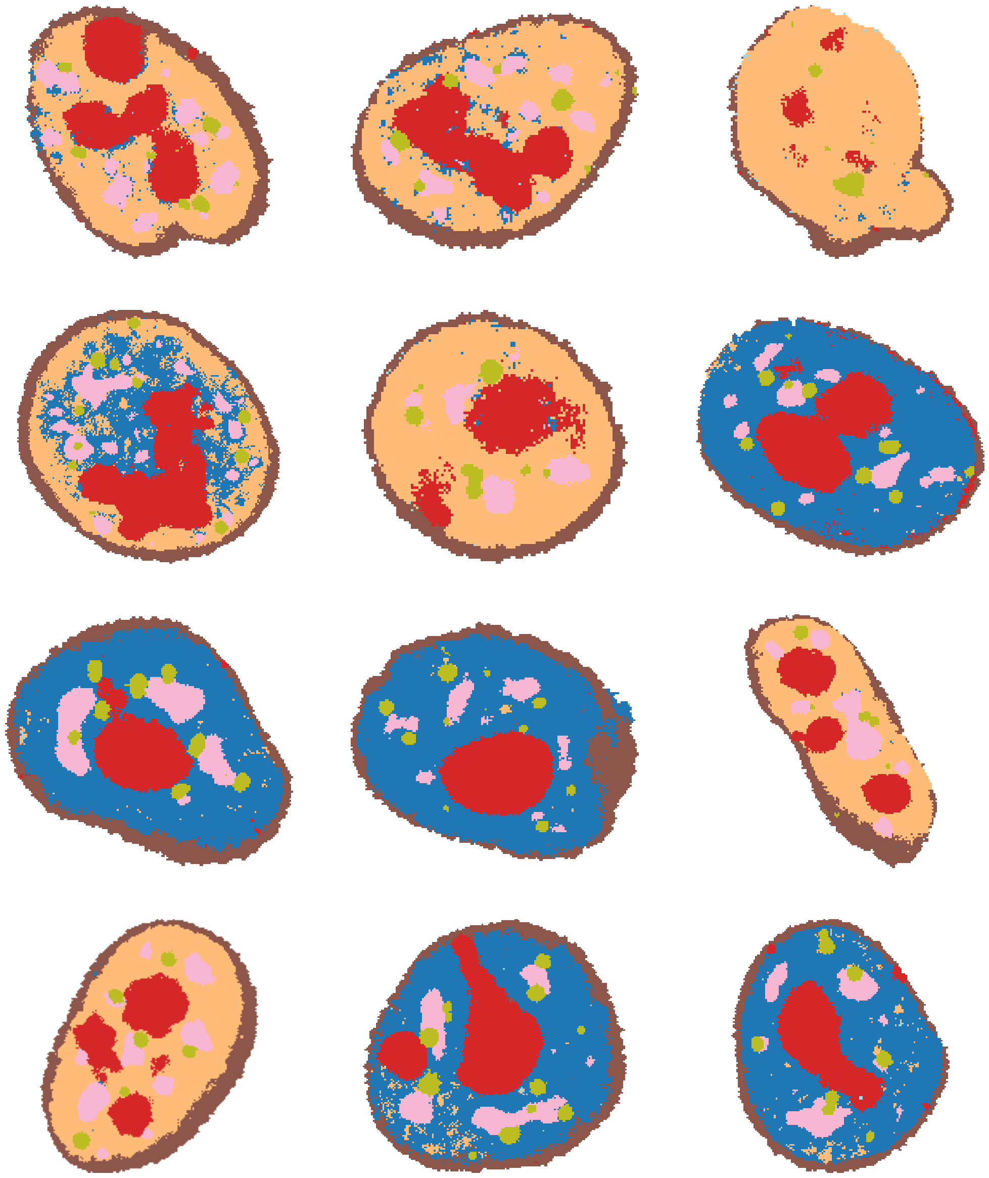
To identify clusters, it can also be very helpful to plot the clusters directly out over some example cells. Using load_full_data_dict and get_clustered_cells, we can cluster some random cells from each well of the experiment.

[14]:

# NOTE: this may take a couple of minutes
# load data
exp = Experiment.from_dir("test_pre_trained/CondVAE_pert-CC")
mpp_datas = load_full_data_dict(exp)
# project clustering to some example cells
example_cells = {}
example_cells.update(get_clustered_cells(mpp_datas, cl, "clustering_res0.2", num_objs=3))

184A1_unperturbed/I09
184A1_unperturbed/I11
184A1_meayamycin/I12
184A1_meayamycin/I20

[15]:

fig, axes = plt.subplots(4, 3, figsize=(25, 30))
for j, data_dir in enumerate(
    ["184A1_unperturbed/I09", "184A1_unperturbed/I11", "184A1_meayamycin/I12", "184A1_meayamycin/I20"]
):
    for i in range(3):
        axes[j, i].imshow(example_cells["clustering_res0.2_colored"][data_dir][i])

for ax in axes.flat:
    ax.axis("off")

Get subcellular localisation from HPA

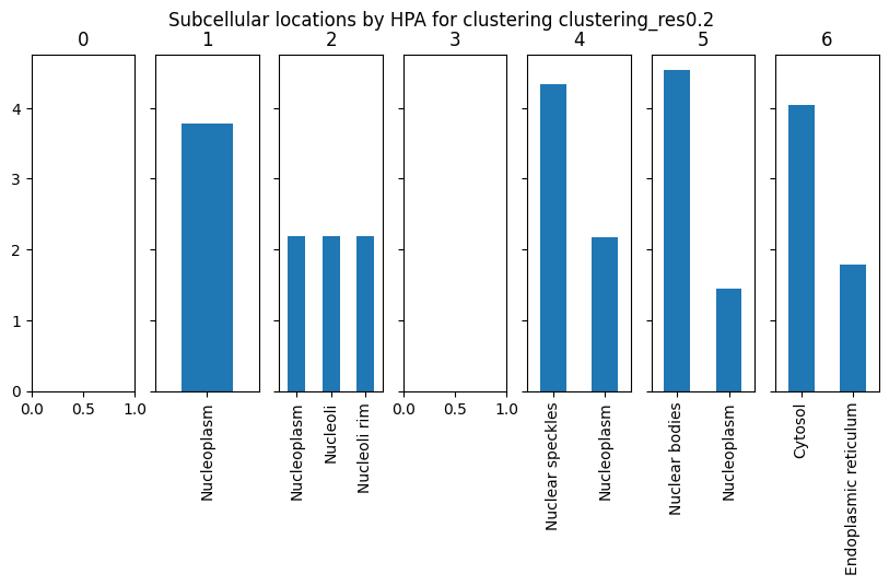
We can also query the Human Protein Atlas to get subcellular locations of the most enriched channels for each protein. For this, we will use Cluster.get_hpa_localisation. This function returns a dictionary of results for each cluster in our data. Here, we set max_num_channels to 3 to get a location information from the top 3 most enriched channels per cluster (weighted by z-scored channel intensity).

[16]:

cluster_name = "clustering_res0.2"
results = cl.get_hpa_localisation(
    cluster_name=cluster_name, thresh=1, max_num_channels=3, limit_to_groups={"perturbation_duration": "normal"}
)

This function returns a dictionary for each cluster containing the genes that were used to query HPA for subcellular location and the query results. The results dictionary is empty if no enriched channels were found for this cluster or if HPA returned no results.

[17]:

# look at results for cluster 1
display(results["1"]["hpa_data"])
print(results["1"]["subcellular_locations"])

	Ensembl	Gene	Gene synonym	Reliability (IF)	Subcellular main location	Subcellular additional location	gene_weights
H2B	ENSG00000184678	H2BC21	[H2B, H2B.1, H2B/q, H2BE, H2BFQ, HIST2H2BE]	Approved	[Nucleoplasm]	[Cytosol]	2.114632
KPNA2	ENSG00000182481	KPNA2	[IPOA1, QIP2, RCH1, SRP1alpha]	Enhanced	[Nucleoplasm]	[Cytosol]	1.662806

Nucleoplasm    3.777438
dtype: float64

[18]:

# plot HPA annotation of clusters
fig, axes = plt.subplots(1, len(results), squeeze=False, sharey=True, figsize=(10, 4))
for ax, (idx, res) in zip(axes.flat, results.items()):
    if res["subcellular_locations"] is not None:
        res["subcellular_locations"].plot(kind="bar", ax=ax)
    ax.set_title(idx)
plt.suptitle(f"Subcellular locations by HPA for clustering {cluster_name}")

[18]:

Text(0.5, 0.98, 'Subcellular locations by HPA for clustering clustering_res0.2')

Annotate clustering

Now, we are ready to annotate the clustering with names of the known structures. We will use the HPA subcellular locations, the example images showing the spatial distribution of clusters in cells, and the channel intensities in each cluster plotted above to make a final assignment of clusters to names. Note that this annotation might vary slightly when rerunning this experiment and clustering, due to the inherent randomness of neural network training. As misannotations can introduce a bias in subsequent analysis of the CSLs, we recommend that users only annotate those CSLs where they are sure that this CSL corresponds to the annotated structure.

In this example, we map multiple different clusters to “Nucleoplasm” because we are not especially interested in these different Nucleoplasm ‘flavours’ identified, which tend to occur heterogeneously between cells. This merging process is entirely optional and we recommend that users keep these separate unless they are sure they want to merge. Another possibility is ‘Nucleoplasm 1’, ‘Nucleoplasm 2’ etc.

For the annotation, we will create a dictionary mapping leiden cluster names to annotated names, and use Cluster.add_cluster_annotation to add the annotation to the Cluster object. Annotations and colour maps for the annotations are stored in a csv file in the cluster_data_dir.

[19]:

annotation = {
    # No enriched markers -> nucleoplasm
    "0": "Nucleoplasm",
    # Nucleoplasm (consistent with HPA label)
    "1": "Nucleoplasm",
    # Nucleolus, due to appearance of NCL marker in this cluster.
    # HPA assigns either Nucleoplasm, Nucleoli or Nucleoli rim label
    "2": "Nucleolus",
    # No enriched markers -> nucleoplasm
    "3": "Nucleoplasm",
    # HPA label: Nuclear speckles
    "4": "Nuclear speckles",
    # HPA label: nuclear bodies (= PML bodies).
    "5": "PML bodies",
    # HPA label: cytosol
    # This is a PABPC-1 enriched cluster only occurring on the Meayamycin perturbation (see UMAP)
    # This occurs here, because we did not use enough training data to train a completely perturbation-independent embedding of the data.
    # Let us assign this small cluster of Nucleoplasm for now.
    # Note that in the manuscript, we don't have perturbation-specific clusters in the cVAE output.
    "6": "Nucleoplasm",
}

cl.set_cluster_name("clustering_res0.2")
cl.add_cluster_annotation(annotation, "annotation")

The resulting cluster annotation data frame is stored in cluster_data_dir/clustering_res0.2_annotation.csv

[20]:

# check out the resulting cluster annotation data frame - this is stored in cluster_data_dir/clustering_res0.2_annotation.csv
display(cl.cluster_annotation)
cluster_dir = os.path.join(campa_config.EXPERIMENT_DIR, cl.config["cluster_data_dir"])
print(cluster_dir)
print(os.listdir(cluster_dir))

	clustering_res0.2	clustering_res0.2_colors	annotation	annotation_colors
index
0	0	#1f77b4	Nucleoplasm	#f7b6d2
1	1	#ffbb78	Nucleoplasm	#f7b6d2
2	2	#d62728	Nucleolus	#d62728
3	3	#8c564b	Nucleoplasm	#f7b6d2
4	4	#f7b6d2	Nuclear speckles	#1f77b4
5	5	#bcbd22	PML bodies	#9edae5
6	6	#9edae5	Nucleoplasm	#f7b6d2
7		#ffffff	NaN	#ffffff

/home/icb/hannah.spitzer/projects/pelkmans/software_new/campa_notebooks_test/example_experiments/test_pre_trained/CondVAE_pert-CC/aggregated/sub-pre
['channels.csv', 'labels.npy', 'latent.npy', 'y.npy', 'conditions.npy', 'umap.npy', 'mpp.npy', 'pynndescent_index.pickle', 'obj_ids.npy', 'cluster_params.json', 'clustering_res0.2_annotation.csv', 'clustering_res0.2.npy', 'metadata.csv', 'x.npy']

[21]:

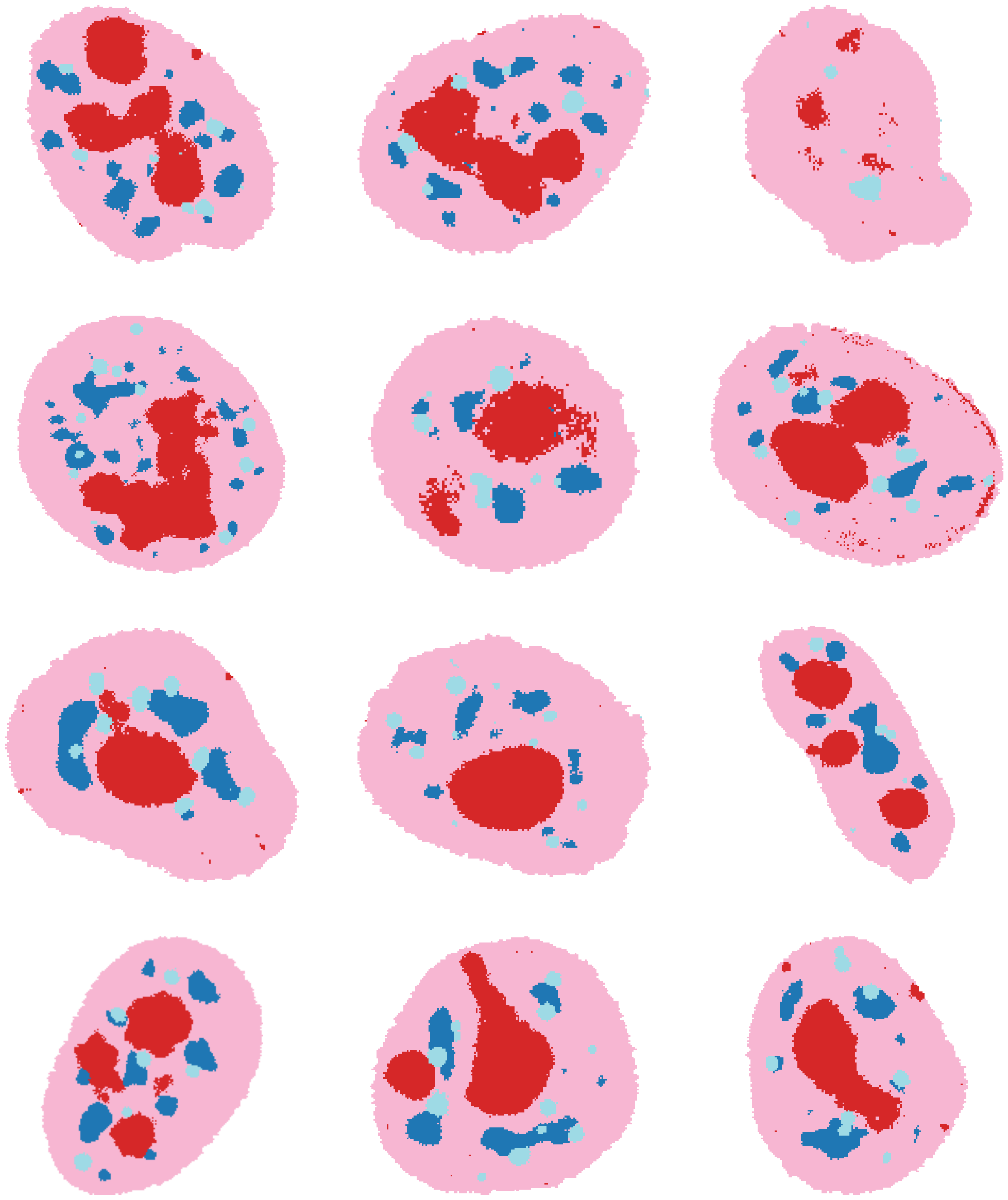
# check out cell colored by new annotation
fig, axes = plt.subplots(4, 3, figsize=(25, 30))
for j, data_dir in enumerate(
    ["184A1_unperturbed/I09", "184A1_unperturbed/I11", "184A1_meayamycin/I12", "184A1_meayamycin/I20"]
):
    for i in range(3):
        axes[j, i].imshow(
            annotate_img(
                example_cells["clustering_res0.2"][data_dir][i],
                annotation=cl.cluster_annotation,
                from_col=cl.config["cluster_name"],
                to_col="annotation",
                color=True,
            )
        )

for ax in axes.flat:
    ax.axis("off")

[22]:

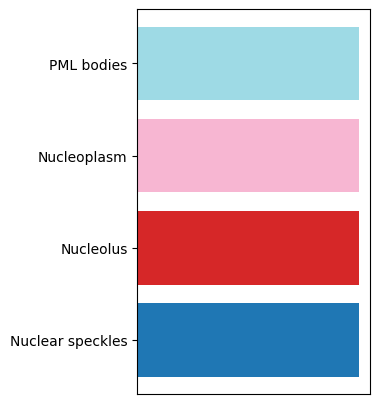
# legend
plt.rcParams["figure.figsize"] = [3, 5]
df = cl.cluster_annotation.groupby("annotation")["annotation_colors"].first()
plt.barh(y=range(len(df)), width=1, color=df)
_ = plt.yticks(range(len(df)), df.index, rotation=0)
_ = plt.xticks([])

Predict model on full data

After generating a clustering on a subset of the data, we can now project it to the entire dataset. For this, the high-level API function project_cluster_data can be used. Alternatively, the CLI can be used:

cd CAMPA_DIR/params
campa cluster test/CondVAE_pert-CC project aggregated/sub-pre --save-dir aggregated/full_data --cluster-name clustering_res0.2

[23]:

project_cluster_data(
    "test_pre_trained/CondVAE_pert-CC",
    cluster_data_dir="aggregated/sub-pre",
    cluster_name="clustering_res0.2",
    save_dir="aggregated/full_data",
)

Cannot read with memmap:  /home/icb/hannah.spitzer/projects/pelkmans/software_new/campa_notebooks_test/example_experiments/test_pre_trained/CondVAE_pert-CC/aggregated/sub-pre/clustering_res0.2.npy

WARNING:MPPData:Saving partial keys of mpp data without a base_data_dir to enable correct loading
WARNING:MPPData:Saving partial keys of mpp data without a base_data_dir to enable correct loading
WARNING:MPPData:Saving partial keys of mpp data without a base_data_dir to enable correct loading
WARNING:MPPData:Saving partial keys of mpp data without a base_data_dir to enable correct loading

This creates npy files containing the clustering for the full data:

[24]:

# check out the resulting clustering using one data_dir
full_data_dir = "test_pre_trained/CondVAE_pert-CC/aggregated/full_data"
mpp_data = MPPData.from_data_dir(
    os.path.join(campa_config.EXPERIMENT_DIR, full_data_dir, "184A1_unperturbed/I09"),
    data_config="ExampleData",
    keys=["clustering_res0.2"],
)
print("clustering:", mpp_data.data("clustering_res0.2"))

Cannot read with memmap:  /home/icb/hannah.spitzer/projects/pelkmans/software_new/campa_notebooks_test/example_experiments/test_pre_trained/CondVAE_pert-CC/aggregated/full_data/184A1_unperturbed/I09/clustering_res0.2.npy
clustering: ['3' '3' '3' ... '3' '3' '3']

We are now ready to extract molecular, morphological, and size features from the CSLs. This is described in the Extract features from CSLs tutorial.