Data representation

MPPData is the main data representation for pixel-level data used by CAMPA. See also the overview for more information about the on-disk file format.

When possible, MPPData lazily loads the source numpy files (using numpy.memmap). If lazy loading fails, the file will be loaded in memory.

[1]:

from pathlib import Path

from IPython.display import display
import numpy as np
import matplotlib.pyplot as plt

from campa.data import MPPData, load_example_data
from campa.utils import init_logging
from campa.constants import campa_config

# init logging with level INFO=20, WARNING=30
init_logging(level=30)
# ensure that example data is downloaded
load_example_data()
# read correct campa_config -- created with setup.ipynb
CAMPA_DIR = Path.cwd()
campa_config.config_fname = CAMPA_DIR / "params/campa.ini"
print(campa_config)

2022-11-25 10:19:56.178552: I tensorflow/core/platform/cpu_feature_guard.cc:193] This TensorFlow binary is optimized with oneAPI Deep Neural Network Library (oneDNN) to use the following CPU instructions in performance-critical operations:  AVX2 AVX512F AVX512_VNNI FMA
To enable them in other operations, rebuild TensorFlow with the appropriate compiler flags.
2022-11-25 10:19:57.965331: I tensorflow/core/util/util.cc:169] oneDNN custom operations are on. You may see slightly different numerical results due to floating-point round-off errors from different computation orders. To turn them off, set the environment variable `TF_ENABLE_ONEDNN_OPTS=0`.
2022-11-25 10:19:58.277749: E tensorflow/stream_executor/cuda/cuda_blas.cc:2981] Unable to register cuBLAS factory: Attempting to register factory for plugin cuBLAS when one has already been registered

Reading config from /home/icb/hannah.spitzer/projects/pelkmans/software_new/campa_notebooks_test/params/campa.ini
CAMPAConfig (fname: /home/icb/hannah.spitzer/projects/pelkmans/software_new/campa_notebooks_test/params/campa.ini)
EXPERIMENT_DIR: /home/icb/hannah.spitzer/projects/pelkmans/software_new/campa_notebooks_test/example_experiments
BASE_DATA_DIR: /home/icb/hannah.spitzer/projects/pelkmans/software_new/campa_notebooks_test/example_data
CO_OCC_CHUNK_SIZE: 10000000.0
data_config/exampledata: /home/icb/hannah.spitzer/projects/pelkmans/software_new/campa_notebooks_test/params/ExampleData_constants.py

The MPPData class

We can construct the MPPData instance from numpy and csv files (as described in overview) using MPPData.from_data_dir.

Note that the data_dir provided to the function should be relative to base_dir, which is either provided directly in the function or set to data_config.DATA_DIR otherwise.

[2]:

mpp_data = MPPData.from_data_dir("184A1_unperturbed/I09", data_config="ExampleData")
print(mpp_data)

MPPData for ExampleData (247872 mpps with shape (1, 1, 35) from 20 objects). Data keys: ['y', 'obj_ids', 'x', 'mpp', 'labels'].

All data is accessible through MPPData.data, and there are several convenience attributes for faster access. Attributes x and y are spatial coordinates of each data point (pixel), obj_ids map pixels to objects (cells), and mpp contains the multiplexed pixel profiles, a #pixels x #channels vector.

[3]:

print(mpp_data.data("x"))
print(mpp_data.x)
print(mpp_data.y)
print(mpp_data.mpp.shape)

[1448 1452 1453 ... 1768 1769 1770]
[1448 1452 1453 ... 1768 1769 1770]
[ 106  106  106 ... 1832 1832 1832]
(247872, 1, 1, 35)

Note that the shape of the mpp_data is #pixels x 1 x 1 x #channels. This is because we can add a square neighbourbood around each pixel to the mpp_data.

The centre mpp can be accessed using MPPData.center_mpp:

[4]:

print(mpp_data.center_mpp)

[[142 108 166 ... 110 121 144]
 [147 113 136 ... 109 127 146]
 [157 121 118 ... 105 126 145]
 ...
 [180 111 139 ... 109 123 255]
 [157 105 156 ... 115 128 249]
 [137 102 178 ... 113 140 234]]

Metadata is stored in MPPData.metadata and channel information in MPPData.channels

[5]:

display(mpp_data.metadata)
display(mpp_data.channels)

	mapobject_id	plate_name	well_name	well_pos_y	well_pos_x	label	mapobject_id_cell	...	perturbation	secondary_only	siRNA	perturbation_duration	LocalDensity_Nuclei_800	TR_factor	TR_norm	TR	TR_factor_DMSO-unperturbed	TR_norm_DMSO-unperturbed
0	324138	plate01	I09	0	2	3	324079	...	normal	False	NaN	normal	0.000116	0.974852	409.119591	419.673544	0.974852	409.119591
1	291041	plate01	I09	0	3	12	290975	...	normal	False	NaN	normal	0.000190	0.974852	432.410658	443.565445	0.974852	432.410658
2	383793	plate01	I09	0	4	19	383757	...	normal	False	NaN	normal	0.000118	0.974852	366.781820	376.243596	0.974852	366.781820
3	383341	plate01	I09	1	3	49	383287	...	normal	False	NaN	normal	0.000149	0.974852	378.254582	388.012319	0.974852	378.254582
4	345908	plate01	I09	1	4	15	345871	...	normal	False	NaN	normal	0.000118	0.974852	308.057232	316.004105	0.974852	308.057232
5	205776	plate01	I09	2	1	8	205742	...	normal	False	NaN	normal	0.000128	0.974852	348.677269	357.672008	0.974852	348.677269
6	205790	plate01	I09	2	1	22	205756	...	normal	False	NaN	normal	0.000149	0.974852	417.591761	428.364268	0.974852	417.591761
7	256546	plate01	I09	2	3	8	256502	...	normal	False	NaN	normal	0.000138	0.974852	236.845799	242.955649	0.974852	236.845799
8	231620	plate01	I09	2	4	31	231520	...	normal	False	NaN	normal	0.000123	0.974852	117.952101	120.994881	0.974852	117.952101
9	359378	plate01	I09	3	1	19	359333	...	normal	False	NaN	normal	0.000145	0.974852	358.652196	367.904255	0.974852	358.652196
10	359391	plate01	I09	3	1	32	359346	...	normal	False	NaN	normal	0.000126	0.974852	224.221344	230.005525	0.974852	224.221344
11	359393	plate01	I09	3	1	34	359348	...	normal	False	NaN	normal	0.000122	0.974852	500.750849	513.668590	0.974852	500.750849
12	259784	plate01	I09	3	3	29	259737	...	normal	False	NaN	normal	0.000135	0.974852	339.395416	348.150713	0.974852	339.395416
13	331833	plate01	I09	4	0	2	331804	...	normal	False	NaN	normal	0.000132	0.974852	375.379685	385.063259	0.974852	375.379685
14	366486	plate01	I09	4	2	33	366427	...	normal	False	NaN	normal	0.000173	0.974852	339.261575	348.013419	0.974852	339.261575
15	366493	plate01	I09	4	2	40	366434	...	normal	False	NaN	normal	0.000140	0.974852	322.527668	330.847832	0.974852	322.527668
16	200792	plate01	I09	4	3	50	200738	...	normal	False	NaN	normal	0.000155	0.974852	270.571286	277.551145	0.974852	270.571286
17	248082	plate01	I09	5	4	17	248037	...	normal	False	NaN	normal	0.000156	0.974852	244.189292	250.488581	0.974852	244.189292
18	248102	plate01	I09	5	4	37	248057	...	normal	False	NaN	normal	0.000147	0.974852	502.765703	515.735421	0.974852	502.765703
19	248104	plate01	I09	5	4	39	248059	...	normal	False	NaN	normal	0.000086	0.974852	461.598482	473.506220	0.974852	461.598482

20 rows × 44 columns

	name
channel_id
0	00_EU
1	01_CDK9_pT186
2	01_PABPC1
3	02_CDK7
4	03_CDK9
5	03_RPS6
6	05_GTF2B
7	05_Sm
8	07_POLR2A
9	07_SETD1A
10	08_H3K4me3
11	09_CCNT1
12	09_SRRM2
13	10_H3K27ac
14	10_POL2RA_pS2
15	11_KPNA2_MAX
16	11_PML
17	12_RB1_pS807_S811
18	12_YAP1
19	13_PABPN1
20	13_POL2RA_pS5
21	14_PCNA
22	15_SON
23	15_U2SNRNPB
24	16_H3
25	17_HDAC3
26	17_SRSF2
27	18_NONO
28	19_KPNA1_MAX
29	20_ALYREF
30	20_SP100
31	21_COIL
32	21_NCL
33	00_DAPI
34	07_H2B

Export and saving

Save mpp data

The MPPData object can be stored on dist using MPPData.write

Export as csv

Using MPPData.extract_csv, we can extract MPPData into a pandas dataframe.

[6]:

mpp_data.extract_csv(data="mpp", obs=["well_name"])

[6]:

name	00_EU	01_CDK9_pT186	01_PABPC1	02_CDK7	03_CDK9	03_RPS6	05_GTF2B	05_Sm	07_POLR2A	07_SETD1A	...	20_ALYREF	20_SP100	21_COIL	21_NCL	00_DAPI	07_H2B	x	y	well_name	mapobject_id
0	142	108	166	174	106	121	115	113	114	111	...	134	104	110	110	121	144	1448	106	I09	324138
1	147	113	136	153	115	125	109	125	110	109	...	127	110	111	109	127	146	1452	106	I09	324138
2	157	121	118	139	116	114	120	123	116	106	...	128	106	104	105	126	145	1453	106	I09	324138
3	161	113	128	124	116	119	115	118	113	109	...	128	111	111	108	132	138	1454	106	I09	324138
4	158	108	127	114	114	133	113	122	116	112	...	137	108	106	117	131	161	1465	106	I09	324138
...	...	...	...	...	...	...	...	...	...	...	...	...	...	...	...	...	...	...	...	...	...
247867	209	112	157	121	106	147	152	108	118	114	...	184	106	111	115	125	255	1766	1832	I09	248104
247868	161	113	158	126	111	137	122	132	116	115	...	190	102	113	114	120	239	1767	1832	I09	248104
247869	180	111	139	128	103	135	109	123	135	108	...	173	105	108	109	123	255	1768	1832	I09	248104
247870	157	105	156	121	104	156	117	125	135	113	...	167	109	117	115	128	249	1769	1832	I09	248104
247871	137	102	178	125	107	152	120	118	124	116	...	162	106	114	113	140	234	1770	1832	I09	248104

247872 rows × 39 columns

Convert to adata

We can convert the MPPData to an AnnData object, and use scanpy functions for further analysis.

Let us create an adata object for one cell. For that, we first need to subset mpp_data to one cell, and then use MPPData.get_adata to create the AnnData object.

[7]:

# subset to one cell
mpp_data_sub = mpp_data.subset(obj_ids=mpp_data.unique_obj_ids[:1], copy=True)

# get adata object from information in MPPData
adata = mpp_data_sub.get_adata()
print(adata)

AnnData object with n_obs × n_vars = 12494 × 35
    obs: 'mapobject_id', 'plate_name', 'well_name', 'well_pos_y', 'well_pos_x', 'tpoint', 'zplane', 'label', 'is_border', 'mapobject_id_cell', 'plate_name_cell', 'well_name_cell', 'well_pos_y_cell', 'well_pos_x_cell', 'tpoint_cell', 'zplane_cell', 'label_cell', 'is_border_cell', 'is_mitotic', 'is_mitotic_labels', 'is_polynuclei_HeLa', 'is_polynuclei_HeLa_labels', 'is_polynuclei_184A1', 'is_polynuclei_184A1_labels', 'is_SBF2_Sphase_labels', 'is_SBF2_Sphase', 'Heatmap-48', 'cell_cycle', 'description', 'dimensions', 'id', 'cell_type', 'EU', 'duration', 'perturbation', 'secondary_only', 'siRNA', 'perturbation_duration', 'LocalDensity_Nuclei_800', 'TR_factor', 'TR_norm', 'TR', 'TR_factor_DMSO-unperturbed', 'TR_norm_DMSO-unperturbed'
    var: 'name'
    obsm: 'spatial'

The resulting adata object contains pixels as obs and channels as var. It also contains all mpp_data.metadata columns.

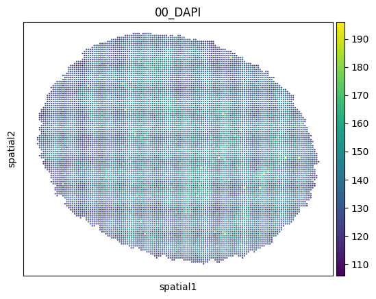
We can now use all scanpy functions on this object, e.g. spatial plotting:

[8]:

import scanpy as sc

sc.pl.embedding(adata, basis="spatial", color=["00_DAPI"])

Visualisation

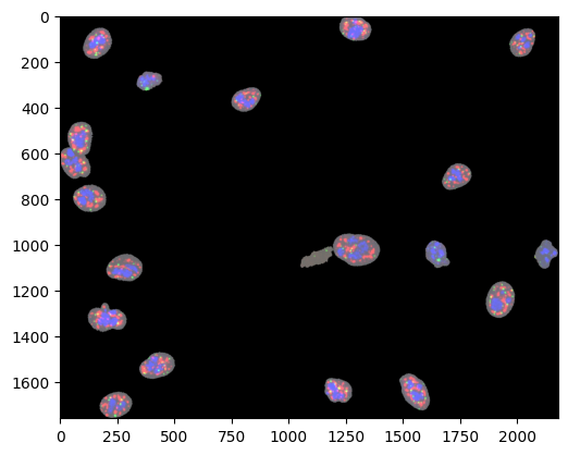
We can visualise several channels of the data of either part of the data or of individual objects (e.g. cells). First, let us plot all objects contained in MPPData with their spatial coordinates x and y using MPPData.get_img.

If you could like to get an image with specific channels, you can specify the channel_ids. The MPPData.get_channel_ids helps to map channel names to ids.

Note that as the mpp values might be larger than 255 for outliers, we use np.clip to bring all values in the range from 0-255 for plotting.

[9]:

channel_ids = mpp_data.get_channel_ids(["09_SRRM2", "11_PML", "21_NCL"])
print(channel_ids)

img, (offset_x, offset_y) = mpp_data.get_img(
    channel_ids=channel_ids,
)
_ = plt.imshow(np.clip(img, 0, 255))

[12, 16, 32]

This function returns the reconstructed image and offset information that needs to be subtracted from x and y before being able to use them to index the image.

Note that the offset information is only returned when the img_size argument to MPPData.get_img is not defined.

[10]:

print(offset_x, offset_y)

print("Location of first data point in img:", mpp_data.x[0] - offset_x, mpp_data.y[0] - offset_y)
print("Value of img at that location:", img[mpp_data.y[0] - offset_y, mpp_data.x[0] - offset_x])
print("Value of fist data point in mpp for channel_ids:", mpp_data.center_mpp[0, channel_ids])

182 106
Location of first data point in img: 1266 0
Value of img at that location: [104 107 110]
Value of fist data point in mpp for channel_ids: [104 107 110]

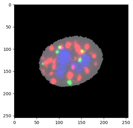
Now let’s plot a single object (cell). For that, MPPData.get_object_img is used.

[11]:

img = mpp_data.get_object_img(mpp_data.unique_obj_ids[0], channel_ids=channel_ids, img_size=255)
_ = plt.imshow(np.clip(img, 0, 255))

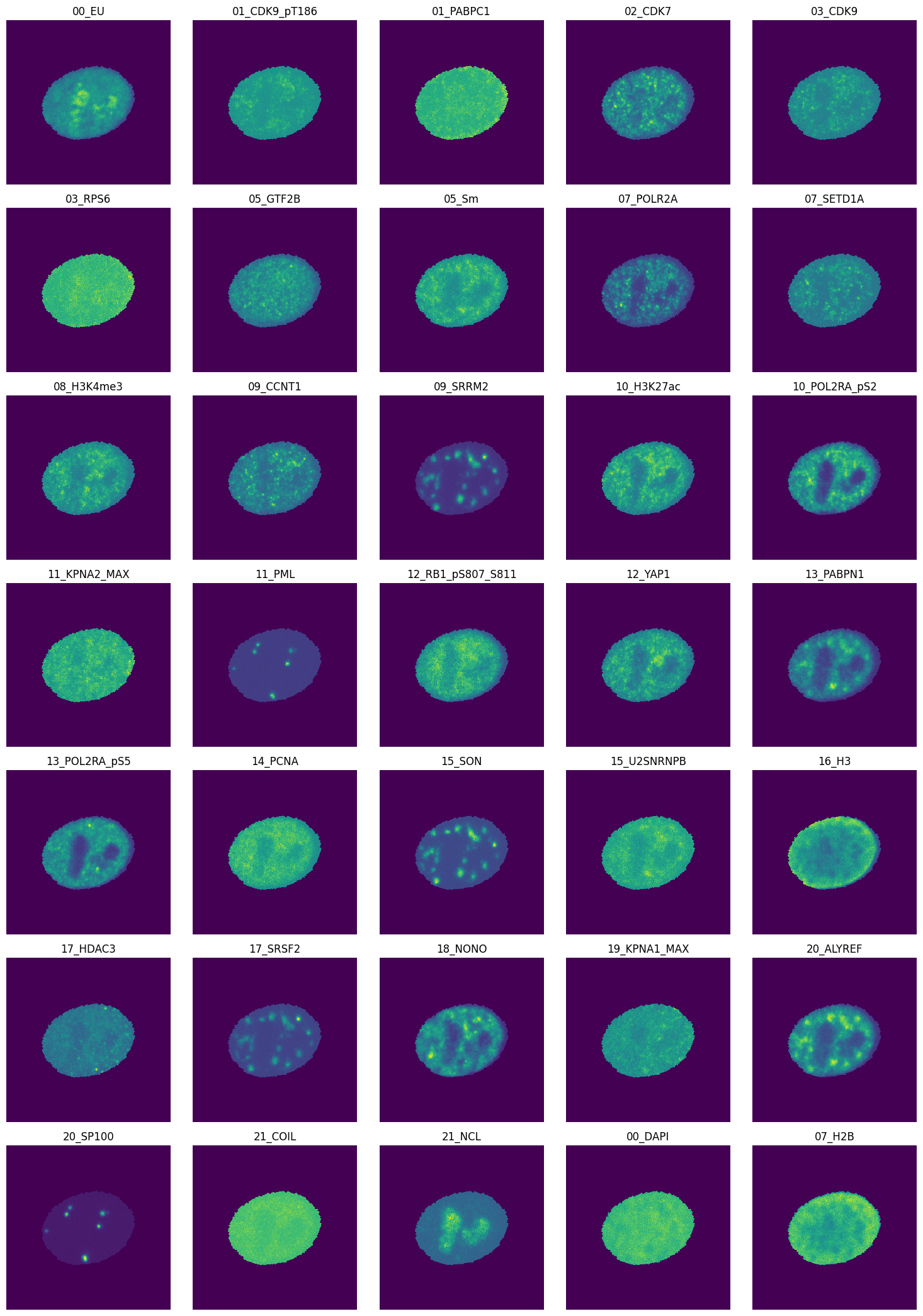
We can also plot all channels of this cell:

[12]:

img = mpp_data.get_object_img(mpp_data.unique_obj_ids[0], img_size=255)
print(img.shape)
num_cols = 5
num_channels = len(mpp_data.channels)
num_rows = num_channels // num_cols

fig, axes = plt.subplots(ncols=num_cols, nrows=num_rows, figsize=(int(3 * num_cols), int(3 * num_rows)))
i = 0
for row in range(num_rows):
    for col in range(num_cols):
        if i >= num_channels:
            break
        axes[row][col].imshow(img[:, :, i], interpolation="none")
        axes[row][col].set_title(mpp_data.channels.iloc[i]["name"])
        axes[row][col].axis("off")
        i += 1
plt.tight_layout()
plt.show()

(255, 255, 35)

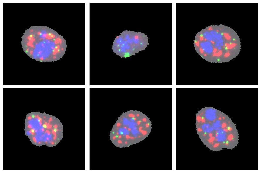
One can also get a list of images for all objects in MPPData using MPPData.get_object_imgs. Let’s get images for all available cells and plot first six:

[13]:

img = mpp_data.get_object_imgs(channel_ids=channel_ids, img_size=255)
num_rows, num_cols = 2, 3
fig, axes = plt.subplots(num_rows, num_cols, figsize=(int(3 * num_cols), (int(3 * num_rows))))
i = 0
for row in range(num_rows):
    for col in range(num_cols):
        axes[row][col].imshow(np.clip(img[i], 0, 255), interpolation="none")
        axes[row][col].axis("off")
        i += 1
plt.tight_layout()
plt.show()
plt.close()

Filter and subset data

There are several functions that allow the modification of mpp_data objects

By channels

We can subset mpp_data selected channels. Note that this operation is performed in-place and will update fields mpp_data.mpp and mpp_data.channels.

[14]:

# subset channels
channels = [
    "01_CDK9_pT186",
    "01_PABPC1",
    "02_CDK7",
    "03_CDK9",
    "03_RPS6",
    "00_DAPI",
    "07_H2B",
]

mpp_data.subset_channels(channels)

print(mpp_data.mpp.shape)
display(mpp_data.channels)

(247872, 1, 1, 7)

	name
channel_id
0	01_CDK9_pT186
1	01_PABPC1
2	02_CDK7
3	03_CDK9
4	03_RPS6
5	00_DAPI
6	07_H2B

By objects (cells)

To filter mpp_data based on specific objects (cells), we use the MPPData.subset function. Several filters for sub-setting can be defined:

subset to random fraction / number of objects
filtering by object ids
filtering by values in MPPData.metadata
filtering by condition values

Subset to random fraction / number of objects

Using attributes frac and num, we can subset the MPPData to a random selection of objects.

[15]:

# Subset fraction of objects:
mpp_data_sub = mpp_data.subset(frac=0.05, copy=True)
print(f"Subset fraction: {len(mpp_data_sub.unique_obj_ids)/len(mpp_data.unique_obj_ids)}")

# Subset specific number of objects:
mpp_data_sub = mpp_data.subset(num=10, copy=True)
print(f"Subset fraction: {len(mpp_data_sub.unique_obj_ids)/len(mpp_data.unique_obj_ids)}")

Subset fraction: 0.05
Subset fraction: 0.5

filtering by object ids

Use obj_ids to select specific objects.

[16]:

# subset to one cell
mpp_data_sub = mpp_data.subset(obj_ids=mpp_data.unique_obj_ids[:1], copy=True)
print(mpp_data.unique_obj_ids)
print(mpp_data_sub.unique_obj_ids)

[200792 205776 205790 231620 248082 248102 248104 256546 259784 291041
 324138 331833 345908 359378 359391 359393 366486 366493 383341 383793]
[200792]

filtering by values in MPPData.metadata

MPPData.metadata contains object-level metadata like e.g. cell cycle state or perturbation status. We can use this information to subset the MPPData.

For that, we need to specify the name of the column in the metadata table and a set of allowed entries for that column. A special entry NO_NAN is a special token selecting all values except NaN values.

We can also provide several columns together with their entries, separated by a comma, and the resulting MPPData object will be computed as a combination of all provided conditions.

[17]:

# filter by NO_NAN cellcycle stage
# perform operation inplace
print(
    "Cell cycle entries before subsetting by NO_NAN values:",
    (mpp_data.metadata.cell_cycle).unique(),
)
mpp_data.subset(cell_cycle="NO_NAN")
print(
    "Cell cycle entries after subsetting to NO_NAN values:",
    np.unique(mpp_data.metadata.cell_cycle),
)

Cell cycle entries before subsetting by NO_NAN values: [nan 'G1' 'G2' 'S']
Cell cycle entries after subsetting to NO_NAN values: ['G1' 'G2' 'S']

By pixels

We can also subset the MPPData by selecting random pixels. For this, the function MPPData.subsample can be used. This is an important step when selecting training data for the cVAE, as we would like to choose samples from all cells, but not necessarily the whole cell (to keep the size of the training data manageable).

[18]:

mpp_data_sub = mpp_data.subsample(frac_per_obj=0.05)

print(f"Subset fraction: {mpp_data_sub.mpp.shape[0]/mpp_data.mpp.shape[0]}")

Subset fraction: 0.04996453416108649

Normalisation

To prepare the data, pixel values can be normalised. For that, pixel values can be e.g. shifted and re-scaled so that they end up ranging between 0 and 1. For this, we can use MPPData.normalise. This can do the following:

background normalisation: shift all values by a fixed background value / one background value per channel.
percentile normalisation

Note that the argument rescale_values can be modified as a side-effect by this function. If an empty list is passed as rescale_values, it will be filled with the percentiles calculated on this data. If rescale_values contains previously calculated percentiles, they will be used to re-scale the data, instead of calculating percentiles.

To demonstrate this, let us split the MPPData in two, and first calculate the percentile on the first half.

[19]:

mpp_data1 = mpp_data.subset(obj_ids=mpp_data.unique_obj_ids[:6], copy=True)
mpp_data2 = mpp_data.subset(obj_ids=mpp_data.unique_obj_ids[6:], copy=True)

rescale_values = []
mpp_data1.normalise(percentile=95, rescale_values=rescale_values)
print("Rescale values for mpp_data1:", rescale_values)

Rescale values for mpp_data1: [144.0, 166.0, 319.0, 181.0, 151.0, 167.0, 361.0]

Now, let us use the rescale_values to scale mpp_data2:

[20]:

mpp_data2.normalise(percentile=95, rescale_values=rescale_values)

print("Median in mpp_data1:", np.median(mpp_data1.center_mpp, axis=0))
print("Median in mpp_data2:", np.median(mpp_data2.center_mpp, axis=0))

Median in mpp_data1: [0.8125     0.76506025 0.63009405 0.7016575  0.8476821  0.83233535
 0.72853184]
Median in mpp_data2: [0.8055556  0.7409639  0.6238245  0.70718235 0.8344371  0.83832335
 0.8504155 ]

Prepare for VAE training

In order to prepare data for VAE training, MPPData contains several functions for - adding neighbourhood information - addition conditions - splitting data in train/val/test

Neighbourhood information

For the CAMPA workflow, it is advantageous to add a small local neighbourhood to each pixel. This results in a more stable latent space. To add neighbourhood information, use the MPPData.add_neighborhood function. Note that this only works before we do any random subsampling of pixels.

It is also possible to do subsampling and add neighbourhood information at the same time using the add_neighborhood argument of the MPPData.subsample function. This is more time-efficient, as the neighbours only need to be computed for every subsampled pixel.

[21]:

mpp_data_neighb = mpp_data.add_neighborhood(size=3, copy=True)

print(f"MPP dataset before adding the neighbourhood, has neighbour data: {mpp_data.has_neighbor_data}")
print(f"Representation of one MPP before adding the neighbourhood (first channel):\n {mpp_data.mpp[0,:, :, 0]}")

print(f"MPP dataset after adding the neighbourhood, has neighbor data: {mpp_data_neighb.has_neighbor_data}")
print(f"Representation of one mpp after adding the neighbourhood (first channel):\n {mpp_data_neighb.mpp[0, :, :, 0]}")

MPP dataset before adding the neighbourhood, has neighbour data: False
Representation of one MPP before adding the neighbourhood (first channel):
 [[117]]
MPP dataset after adding the neighbourhood, has neighbor data: True
Representation of one mpp after adding the neighbourhood (first channel):
 [[117 117 117]
 [117 117 117]
 [111 116 123]]

[22]:

# subsample and add neighbourhood

mpp_data_sub = mpp_data.subsample(frac_per_obj=0.05, add_neighborhood=True, neighborhood_size=3)

print(f"Subset fraction: {mpp_data_sub.mpp.shape[0]/mpp_data.mpp.shape[0]}")

print(f"MPP representation before adding the neighbourhood (first channel)\n: {mpp_data.mpp[0,:, :, 0]}")
print(f"MPP representation after adding the neighbourhood (first channel)\n: {mpp_data_sub.mpp[0, :, :, 0]}")

Subset fraction: 0.04996453416108649
MPP representation before adding the neighbourhood (first channel)
: [[117]]
MPP representation after adding the neighbourhood (first channel)
: [[114 126 109]
 [121 124 122]
 [125 127 119]]

Note that since a random subsampling was performed, the first value in the mpp_data does not necessarily correspond to the first element in mpp_data_sub.

Add conditions to MPPData

The CAMPA framework allows you to learn a condition-independent latent representation of input pixel profiles. For this, we are training a conditional VAE. Here, we are going to prepare the MPPData for this by adding a special condition vector, MPPData.conditions to the object. This could represent e.g. perturbation or cell cycle.

MPPData.add_conditions prepares and adds this condition vector, utilising cell-level information from the MPPData.metadata table. Before categorical conditions can be added, they need to be described on data_config.CONDITIONS, to enable a mapping from categorical values to numbers.

cond_desc describes the conditions that should be added. It is a list of condition descriptions. Each condition is calculated separately and concatenated to form the resulting MPPData.conditions vector. Condition descriptions have the following format: "{condition}(_{postprocess})".

Condition values are obtained as follows:

look up condition in MPPData.metadata. If condition is described in data_config.CONDITIONS, map it to numerical values. Note that if there is an entry UNKNOWN in data_config.CONDITIONS, all unmapped values will be mapped to this class. If condition is not described in data_config.CONDITIONS, values are assumed to be continuous and stored as they are in the condition vector.
post-process conditions. postprocess can be one of the following values:
- lowhigh_bin_2: Only for continuous values. Removes middle values. Bin all values in 4 quantiles, encodes values in the lowest quantile as one class and values in the high quantile as the second class (one-hot encoded), and set all values in between set to NaN.
- bin_3: Only for continuous values. Bin values in .33 and .66 quantiles and one-hot encode each value.
- zscore: Only for continuous values. Normalise values by mean and std.
- one_hot: Only for categorical values. One-hot encode values.

For categorical descriptions, it is possible to pass a list of condition descriptions. This will return a unique one-hot encoded vector combining multiple conditions.

We can also provide a cond_params dict to the function, to enable the use of precomputed quantiles or mean/std values. If no values are provided in cond_params, the computed quantiles or mean/std values are added to cond_params, allowing us to use these values to process other MPPData objects.

In the following, let us look at some examples how to add conditions.

Continuous conditions

Let us use the transcription rate condition TR for this example. Remember, that every condition we are adding needs to be present in the MPPData.metadata table.

For this dataset, we computed the transcription rate as mean EU molecular intensity per cell over a period of 30 minutes. This gives an estimate of the amount of new RNA transcripts.

Let us again split the MPPData and first add conditions on this first half

[23]:

mpp_data1 = mpp_data.subset(obj_ids=mpp_data.unique_obj_ids[:6], copy=True)
mpp_data2 = mpp_data.subset(obj_ids=mpp_data.unique_obj_ids[6:], copy=True)

cond_params = {}
mpp_data1.add_conditions(["TR_norm_lowhigh_bin_2"], cond_params=cond_params)

print("cond_params for mpp_data1:", cond_params)

cond_params for mpp_data1: {'TR_norm_lowhigh_bin_2_quantile': [339.39541649462217, 417.5917605897343]}

This adds a #pixels x 2 conditions vector to mpp_data1. The two conditions are low quantile TR cells, and high quantile TR cells. All cells that have a TR between the low and high quantiles have NaN values.

As conditions are the same for all pixels in the same cell, we can get an overview over the assigned conditions looking at one value per object id:

[24]:

for obj_id, i in zip(*np.unique(mpp_data1.obj_ids, return_index=True)):
    # get TR for comparison
    TR = float(mpp_data1.metadata[mpp_data1.metadata["mapobject_id"] == obj_id]["TR"])
    # print condition and TR for this cell
    print("obj_id:", obj_id, "condition:", mpp_data1.conditions[i], "TR:", TR)

obj_id: 205776 condition: [nan nan] TR: 357.67200760901375
obj_id: 205790 condition: [1. 0.] TR: 428.3642683585313
obj_id: 248082 condition: [1. 0.] TR: 250.4885806253832
obj_id: 248102 condition: [0. 1.] TR: 515.7354206855616
obj_id: 259784 condition: [1. 0.] TR: 348.1507131885012
obj_id: 291041 condition: [0. 1.] TR: 443.565445026178

We can now use cond_params to use the same quantiles when adding conditions to mpp_data2.

[25]:

mpp_data2.add_conditions(["TR_norm_lowhigh_bin_2"], cond_params=cond_params)

# show resulting conditions
for obj_id, i in zip(*np.unique(mpp_data2.obj_ids, return_index=True)):
    # get TR for comparison
    TR = float(mpp_data2.metadata[mpp_data2.metadata["mapobject_id"] == obj_id]["TR"])
    # print condition and TR for this cell
    print("obj_id:", obj_id, "condition:", mpp_data2.conditions[i], "TR:", TR)

obj_id: 345908 condition: [1. 0.] TR: 316.0041054648299
obj_id: 359378 condition: [nan nan] TR: 367.90425531914894
obj_id: 359393 condition: [0. 1.] TR: 513.66859045505
obj_id: 366493 condition: [1. 0.] TR: 330.84783201527136
obj_id: 383341 condition: [nan nan] TR: 388.0123185637892
obj_id: 383793 condition: [nan nan] TR: 376.2435963681996

Categorical conditions

Categorical conditions are e.g. perturbation or cell cycle. They need to be defined in data_config.CONDITIONS to enable mapping from string values to classes.

Lets check which conditions are defined for this example: Remember that you can add conditions by editing the data_config file.

[26]:

print("data_config:", mpp_data.data_config_name)
print("data_config fname:", campa_config.data_configs[mpp_data.data_config_name.lower()])
print(mpp_data.data_config.CONDITIONS)

data_config: ExampleData
data_config fname: /home/icb/hannah.spitzer/projects/pelkmans/software_new/campa_notebooks_test/params/ExampleData_constants.py
{'perturbation_duration': ['AZD4573-120', 'AZD4573-30', 'CX5461-120', 'DMSO-120', 'DMSO-720', 'Meayamycin-720', 'TSA-30', 'Triptolide-120', 'Wnt-C59-720', 'normal'], 'cell_cycle': ['M', 'G1', 'S', 'G2'], 'well_name': ['H06', 'H07', 'I03', 'I08', 'I09', 'I10', 'I11', 'I12', 'I13', 'I14', 'I16', 'I17', 'I18', 'I20', 'J06', 'J07', 'J08', 'J09', 'J10', 'J12', 'J13', 'J14', 'J15', 'J16', 'J18', 'J20', 'J21', 'J22'], 'siRNA': ['scrambled', 'SBF2']}

Lets use the cell_cycle condition first. Using just cell_cycle as condition will add values between 0-3 (1-3 for this example, as there are no M-stage cells in this data).

[27]:

mpp_data.add_conditions(["cell_cycle"])

print(mpp_data.conditions.shape)
print(np.unique(mpp_data.conditions))

(153669, 1)
[1 2 3]

Using cell_cycle_one_hot will one-hot encode the cell-cycle stage:

[28]:

mpp_data.add_conditions(["cell_cycle_one_hot"])

print(mpp_data.conditions.shape)
print(mpp_data.conditions)

(153669, 4)
[[0. 1. 0. 0.]
 [0. 1. 0. 0.]
 [0. 1. 0. 0.]
 ...
 [0. 0. 1. 0.]
 [0. 0. 1. 0.]
 [0. 0. 1. 0.]]

Combine multiple categorical conditions

We can also combine multiple categorical conditions into one one-hot encoded vector. Here, let us combine cell-cycle and perturbation-duration into one conditions. There are 4 cell-cycle values and 10 perturbation values. This means that there are \(4*10=40\) unique cell-cycle-perturbation combinations, which will result in a #pixels x 40 conditions vector.

[29]:

mpp_data.add_conditions([["cell_cycle_one_hot", "perturbation_duration_one_hot"]])
print(mpp_data.conditions.shape)
print(mpp_data.conditions)

(153669, 40)
[[0. 0. 0. ... 1. 0. 0.]
 [0. 0. 0. ... 1. 0. 0.]
 [0. 0. 0. ... 1. 0. 0.]
 ...
 [0. 0. 0. ... 0. 1. 0.]
 [0. 0. 0. ... 0. 1. 0.]
 [0. 0. 0. ... 0. 1. 0.]]

Combine multiple conditions (concatenation)

Add more condition descriptions to the cond_desc list to combine multiple conditions. Here, we combine the TR value with the one-hot encoded cell-cycle.

The first value is the TR, and the following 4 encode the cell cycle stage.

[30]:

mpp_data.add_conditions(["TR", "cell_cycle_one_hot"])
print(mpp_data.conditions.shape)
print(mpp_data.conditions)

(153669, 5)
[[443.56544503   0.           1.           0.           0.        ]
 [443.56544503   0.           1.           0.           0.        ]
 [443.56544503   0.           1.           0.           0.        ]
 ...
 [515.73542069   0.           0.           1.           0.        ]
 [515.73542069   0.           0.           1.           0.        ]
 [515.73542069   0.           0.           1.           0.        ]]

Train-val-test split

We can use MPPData.train_val_test_split to split the data into train/val/test sets.

[31]:

train, val, test = mpp_data.train_val_test_split(train_frac=0.8, val_frac=0.1)

print("Train", train)
print("Val", val)
print("Test", test)

Train MPPData for ExampleData (102400 mpps with shape (1, 1, 7) from 9 objects). Data keys: ['y', 'obj_ids', 'x', 'mpp', 'labels', 'conditions'].
Val MPPData for ExampleData (13668 mpps with shape (1, 1, 7) from 1 objects). Data keys: ['y', 'obj_ids', 'x', 'mpp', 'labels', 'conditions'].
Test MPPData for ExampleData (37601 mpps with shape (1, 1, 7) from 2 objects). Data keys: ['y', 'obj_ids', 'x', 'mpp', 'labels', 'conditions'].